Algebraic TopologyNoel Sensei
H-hello class ⭐ my name is Noel and I'll be your algebraic topology 🍩 teacher for this class ~ !!! In fact... I'll be your teacher for all our maths classes (very good). I h-highly recommend you pick up a copy of Hatcher's Algebraic Topology which we'll be following for this course ~ !!
1. Fundamental Group $\pi_1(X)$Section 1 is under construction (╯°□°)╯︵ ┻━┻ The fundamental group is all about loops! It records possible ways to loop around a space in the form of a group that is not necessarily commutative. The chapter will be a very fun topic as we will be looking at a lot of pretty pictures. It will also be the easiest part of the course as we will mostly dealing with low dimensional topological spaces and some basic algebra. In category theory, the fundamental group is a functor $\pi_1 : \mathbf{Top_\ast} \to \mathbf{Grp}$ where $\mathbf{Top_\ast}$ is the category of based spaces $X,x_0$ with morphisms given by basepoint-preserving maps, and $\mathbf{Grp}$ is the canonical category of groups. 1.1. Basic ConstructionsThis section will mainly focus on building up the relevant definitions to construct the fundamental group and provide some basic results from such definitions. Most of the definitions should become very intuitive and second nature to you after a while. We will also show that the fundamental group is invariant up to homotopy equivalence and that $\pi_1(S^1)$, the fundamental group of a circle, is isomorphic to $\Z$ with which we can prove show some interesting theorems. We then conclude this section with a fun application to Borromean rings. Now before we begin, let us introduce some notation we will stick to for this class.
Paths and homotopiesA path in a space $X$ is a map $f: I \to X.$ A homotopy of paths from $f$ to $g$ is a family $f_t:I \to X$ with $f_0=f$ and $f_1=g$ satisfying
An equivalent notation for a homotopy is given by a function $F:I \times I \to X$, $(s,t) \mapsto f_t(s).$ Then we have
Write $f\simeq g$ is there exists a homotopy from $f$ to $g.$ It is a fact that $\simeq$ is an equivalence relation on paths in $X$ starting at $x_0$ and ending at $x_1$, and we will let $[f]$ denote the equivalence class of $f.$ Exercise for you to show that $f\simeq f$ and $f \simeq g \implies g \simeq f.$ To see that $f \simeq g$ and $\g \simeq f$ implies $f \simeq h$, suppose $f_t$ and $g_t$ are homotopies from $f$ to $g$ and from $g$ to $h$ respectively. Then we can define a homotopy $h$ from $f$ to $h$ by
$$
h_t(s) =
\begin{cases}
f_{2t}(s) & t \in [0,\frac 12] \\
g_{2t - 1}(s) & t \in [\frac 12, 1].
\end{cases}
$$
Let $f,g: I \to X$ be paths in $X$ and $f(1)=g(0).$ Their composite is the path $f \cdot g$ (note different order than function composition) with
$$
(f\cdot g)(s) =
\begin{cases}
f(2s) & s \in[0,\frac 12] \\
g(2s-1) & s \in [\frac 12,1].
\end{cases}
$$
Now suppose $f_0 \simeq f_1$ and $g_0 \simeq g_1.$ Then we have $f_0 \cdot g_0 \simeq f_1 \cdot g_1$ (exercise!). A result of this is that path composition is well defined on equivalence classes: $[f] \cdot [g] = [f\cdot g].$ We now have sufficient definitions to define the fundamental group. Fundamental group definitionFix $x_0 \in X.$ A loop in $(X,x_0)$ is a path in $X$ starting and ending at $x_0.$ The fundamental group of $(X,x_0)$ is
$$
\pi_1(X,x_0) = \set{[f] \mid \text{$f$ loop in $(X,x_0)$}}.
$$
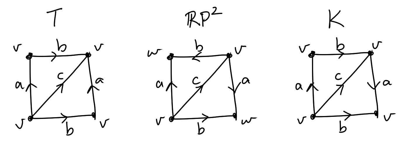
As the name suggests, the fundamental group is a group with product $([f],[g]) \mapsto [f\cdot g]$, identity $e = [c]$ where $c$ is the constant path defined by $c(s) = x_0$ for all $s \in I$, and inverse $[f^{-1}]$ with $f^{-1} = f(1-s).$ Exercise for you to use homotopy definitions to show associativity $([f][g])[h]=[f]([g][h])$, identity $[f][c] = [f] = [c][f]$ and inverse $[f][f^{-1}]=[c].$ Note that the group is not necessary commutative. We will show later for example that the donut $T$ has fundamental group isomorphic to the free group $\Z * \Z.$ The most elementary fundamental group example we can give is $\pi_1(\R^n, x_0) = 0.$ This is because all loops in $\R^n$ are nullhomotopic (homotopic to the constant loop) with homotopy given by linear interpolation. One might ask how $\pi_1(X,x_0)$ depends on $x_0.$ Given a path $h$ from $x_0$ to $x_1$, define a baspoint change homomorphism
\begin{align}
\b_h: \pi_1(X,x_1) &\to \pi_1(X,x_0) \\
[f] &\mapsto [h\cdot f\cdot h^{-1}]
\end{align}
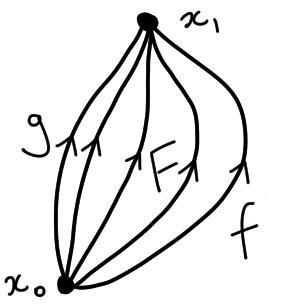
Note that to be pedantic we should have written $(h\cdot f) \cdot h^{-1}$ or $h\cdot(f\cdot h^{-1})$ but these are homotopic. It is a fact that $\b_h$ is an isomorphism of groups with inverse $\b_{h^{-1}}$ (exercise!). A space $X$ is path connected if for all $x_0,x_1 \in X$ there eixsts a path with endpoints $x_0$ and $x_1.$ Thus, if $X$ is path connected, then $\pi_1(X,x_0)$ is independent of $x_0$ up to isomorphism such that in this case we can write $\pi_1(X)$ instead of $\pi_1(X,x_0)$ if we are sure that the choice of $x_0$ does not matter. A space $X$ is simply connected if $X$ is path connected and $\pi_1(X,x_0) = 0$ for some (hence for all) $x_0 \in X.$ Some examples of simply connected spaces are $\R^n, D^n$ for all $n$ and $S^n$ for $n>2.$ $S^0$ is not simply connected since it contains two disjoint points, and $\pi_1(S^1) \cong \Z$ as we will show shortly. Fundamental group is invariant under homotopy equivalenceA homotopy between maps $f,g:X\to Y$ is a family of maps $f_t:X\to Y$ with $f_0 = f$ and $f_1 = g$ such that $F:X \times I \to Y,$ $(x,t) \mapsto f_t(x)$ is continuous. If there exists a homotopy between $f$ and $g$, write $f \simeq g.$ Moreover, $\simeq$ is an equivalence relation on the set of maps from $X$ to $Y.$ $X$ and $Y$ are homeomorphic, denoted $X \cong Y$, if there eixsts $f:X \to Y$ and $g:Y \to X$ with $g\circ f = \id_X$ and $f \circ g = \id_Y.$ $X$ and $Y$ are homotopy equivalent, denoted $X \simeq Y$, if there eixsts $f:X \to Y$ and $g:Y \to X$ with $g\circ f \simeq \id_X$ and $f \circ g \simeq \id_Y.$ Note that homemorphic spaces are homotopy equivalent but not the converse. We also have that homotopy equivalence $\simeq$ is an equivalence relation on the proper class of spaces. $X$ is contractible if $X \simeq *$, where $*$ denotes a one point space. An example is $\R^n$ with $f:\R^n \to *,$ $x\mapsto *$ and $g: * \to \R^n,$ $* \mapsto 0.$ Then $g\circ f \simeq \id_{\R^n}$ by $f_t(x) = tx$ and $f\circ g\simeq \id_*$ since $f \circ g = \id_*.$ Write $(X,x_0)$ for a space $X$ with basepoint $x_0$ and $\phi:(X,x_0) \to (Y,y_0)$ for a map with $\phi(x_0)=y_0.$ Then we get an induced map $\phi_*:\pi_1(X,x_0) \to \pi_1(Y,y_0)$ by $[f]\mapsto [\phi\circ f].$ $\textbf{Theorem 1.1.}$ If $\phi:X\to Y$ is a homotopy equivalence, then $\phi_*: \pi_1(X,x_0) \to \pi_1(Y,\phi(x_0))$ is an isomorphism. $\textit{Proof.}$ Let $\psi:Y \to X$ be the homotopy inverse. Then let $x_1 = \phi(\psi(x_0))$ and $\a_t$ be a homotopy $\id_X \cong \psi \circ \phi.$ Define $h(t) = \a_t(x_0)$ a path from $x_0$ to $x_1.$ Recalling $\b_h$ the change of basis isomorphism, I claim that the following composite is the identity.
$$
\pi_1(X,x_0) \xrightarrow{\phi_*} \pi_1(Y,\phi(x_0)) \xrightarrow{\psi_*} \pi_1(X,x_1) \xrightarrow{\b_h} \pi_1(X,x_0).
$$
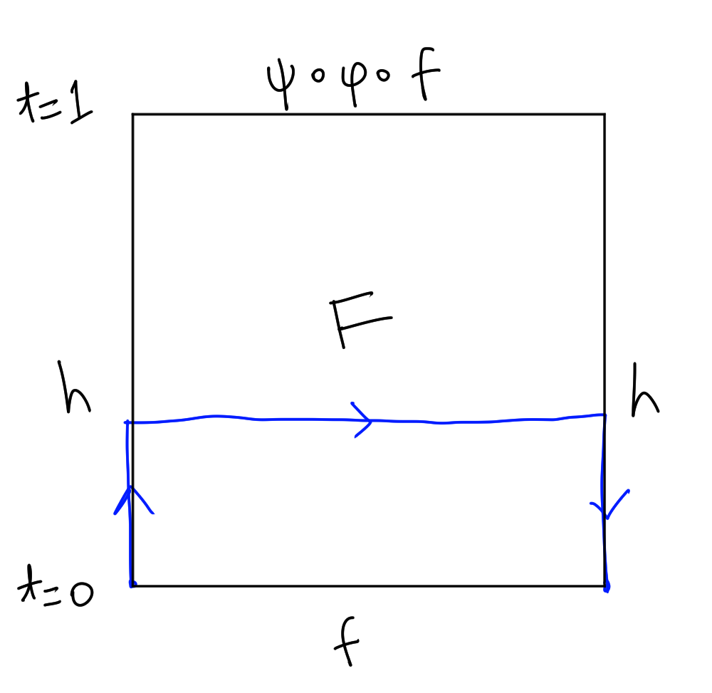
To see this, let $f: I \to X$ be a loop at $x_0$ and $F:I \times I\to X$ a homotopy $(s,t) \mapsto \a_t(f(s)).$ Then $f \simeq h\cdot (\psi \circ \phi \circ f) \cdot h^{-1}$ via
$$
f_t = h\mid_{[0,t]} \cdot F\mid_{I \times \set{t}} \cdot (h\mid_{[0,t]})^{-1}. \quad\Box
$$
Fundamental group of a circle$\textbf{Theorem 1.2.}$ $\pi_1(S^1) \cong \Z.$ $\textit{Proof.}$ $\textbf{Theorem 1.3.}$ (Fundamental Theorem of Algebra) Every nonconstant polynomial with $\C$-coefficients has a root. $\textit{Proof.}$ $\textbf{Theorem 1.4.}$ (Brouwer's Fixed Point Theorem) Any $h:D^2 \to D^2$ has a fixed point. $\textit{Proof.}$ $\textbf{Theorem 1.5.}$ (Borsuk-Ulam Theorem) Given $f:S^2 \to \R^2$, there exists a pair $\set{x,-x}$ with $f(x) = f(-x).$ $\textit{Proof.}$ RetractionsA retraction is a map $r:X\to X$ with $r^2=r.$ If $A = \im(r)$, then $r\mid_A = \id.$ For $A\subset X$, a retraction of $X$ onto $A$ is a map $r : X \to A$ with $r\mid_A = \id.$ Equivalently, a retraction is a map $r: X \to A$ with $r\circ i=\id$ with $i:A \to X$ denoting inclusion. A deformation retraction of $X$ onto $A$ is a homotopy $r_t:X\to X$ from $id_X$ to a retraction. Note that a deformation retraction is a special case of a homotopy equivalence $X \simeq A.$ An example is $M$ a Möbius band deformation retracts onto its central circle $S^1$ by $r_t$ defined below. However, it does not deformation retract onto its boundary circle (exercise using the below proposition!). 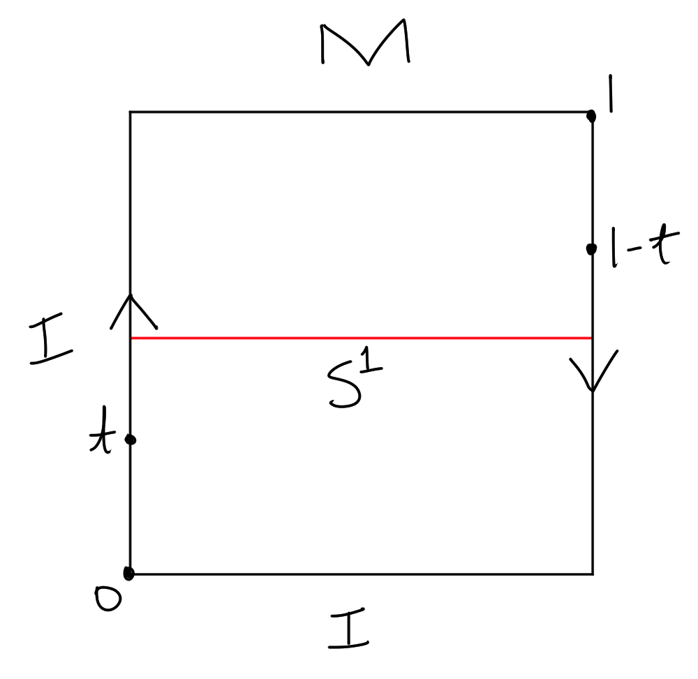
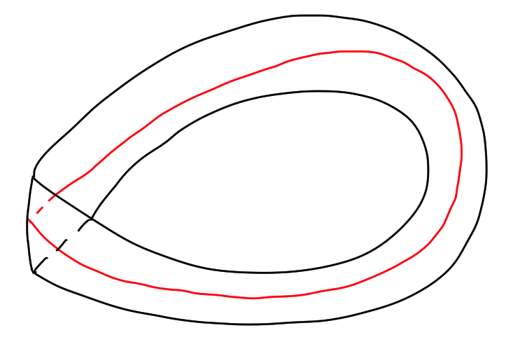
\begin{align}
M = I\times I / (0,t) \sim (1,1-t)
\end{align}
\begin{align}
r_t(x,y) = \lr{x, (1-t)y + t\cdot \frac 12}.
\end{align}
$\textbf{Proposition 1.6.}$
Suppose $A \subset X.$
$\textit{Proof.}$ Since $r\circ i=\id_A$, we have $r_* \circ i_* = \id_{\pi_1(A,x_0)}$ which gives us $i_*$ injective and $r_*$ surjective. For the second statement, let $[f] \in \pi_1(X,x_0).$ Then $r_t \circ f$ is a homotopy from $f$ to $i\circ r \circ f$ which is in the image of $i_*.$ Thus, $[f] = i_*(r_*([f])).$ $\Box$ Exercise: prove Brouwer's fixed point theorem by contradiction by considering $r:D^2 \to S^1$ as defined before as a retraction. 
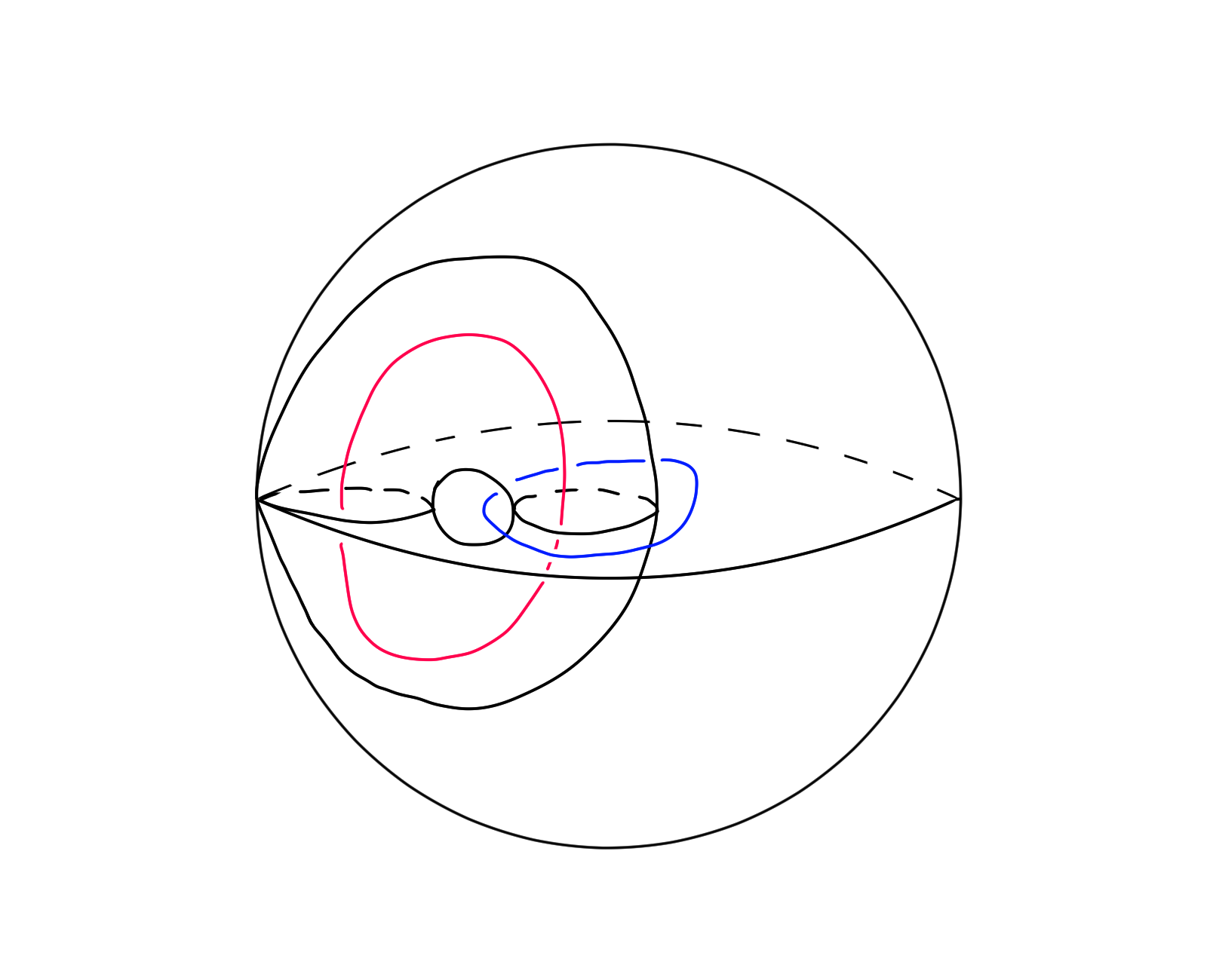
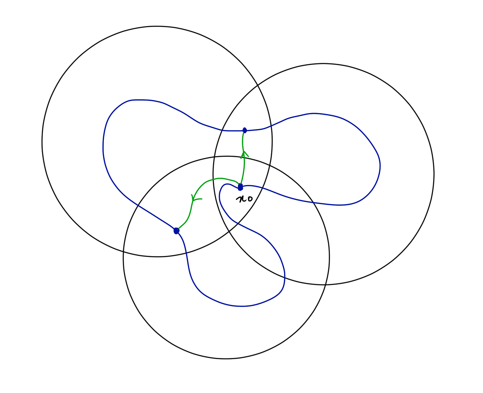
Now let us begin talking about Borromean rings. This is the union of 3 circles in $\R^3$ interlinked in such a way that if you remove one of them the other two become unlinked. We will use algebraic topology to show that Borromean rings generalise, meaning that we can construct unions of $n$ circles for arbitrary $n$ with this linking property. The proof of this will use some definitions and a result in Section 1.2 which we will just state. Feel free to skip this section and come back later, but I have put this example here because it is very fun. First let us consider a ring as a loop $\o$ in the complement of the other two rings $A$ and $B$ and find what element in the fundamental group it represents. We have that $\R^3 \setminus (A \cup B)$ deformation retracts to the wedge sum of two circles and two spheres ($S^1 \vee S^1 \vee S^2 \vee S^2$) whose fundamental group is the free group $\Z * \Z$ with generators $a$ and $b.$ 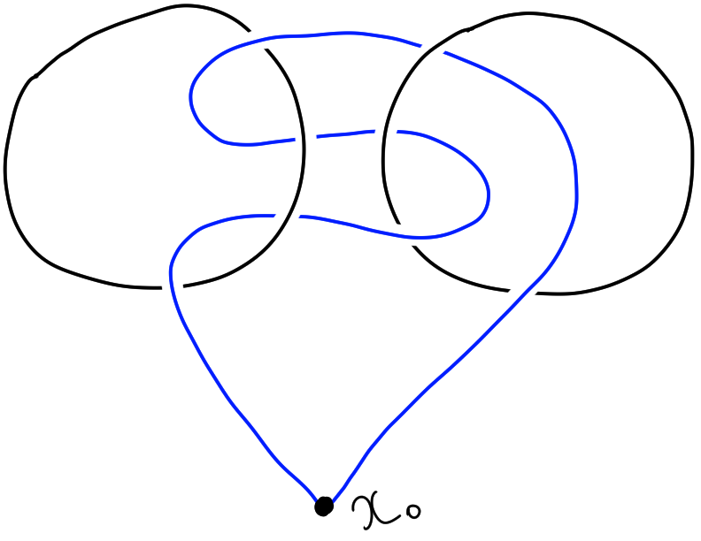
Now I claim that $\o = aba^{-1}b^{-1}.$ Exercise for you to convince yourself this is true with the diagram here. Note that this is the commutator of $a$ and $b$ denoted $[a,b].$ Now we can use group theory to give a way to construct Borromean rings with $n$ rings. Specifically, we can define how to link the $n$th ring by associating it as a loop in the complement of $n-1$ rings in $\R^3$ which we deonte $X.$ Specifically, let $\o = [a_1,[a_2,\ldots[a_{n-2},a_{n-1}]\ldots]]$ where $a_i$ is the $i$th generator of $\pi_1(X)$ now the free group of $n-1$ copies of $\Z.$ 1.2. Van Kampen's TheoremThis section will go over lots of topological spaces and techniques to compute them. wedge sum 1.3. Covering Spaces
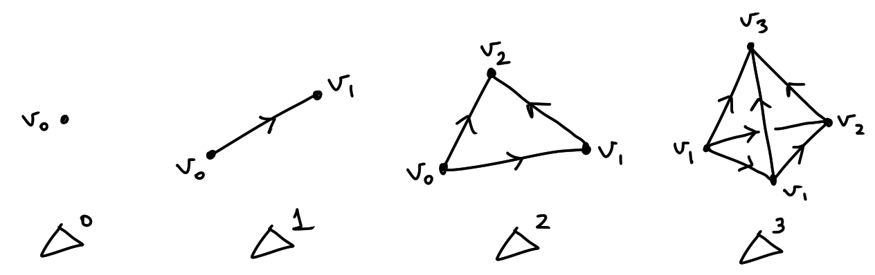
2. Homology $H_n(X)$Homology is all about holes! Homology is better to work with than fundamental groups because they can record higher dimension information of a topological space and because homology groups are abelian. There are actually several variants of homology which we can show are all equivalent. The homology flavours we will look at for this course are simplicial, singular, and cellular homology. In category theory language, homology is a functor $H_*: \mathbf{Top} \to \mathbf{GrAb}$ where we are now dealing with unbased topological spaces, and $\mathbf{GrAb}$ denotes the category of graded abelian groups. 2.1. Simplicial and Singular HomologyThis chapter will look at simplicial and singular homology. The former is easier to visualise and understand, but the latter is better to use for proving general theorems. However, they are both equivalent so it is possible to interchange between the two. Homology definitionsSimplicial homology is defined in three steps:
Singular homology is a bit different with the definition of simplex. It is more flexible as our spaces no longer have to be $\Delta$-complexes.
Maps between spaces induce maps between homologyNow we aim to show that a map between topological spaces induces a map between homology. Define a chain complex $C_*$ as a sequence of maps of abelian groups
\begin{CD}
\ldots @>>> C_{n+1} @>d_{n+1}>> C_n @>d_{n}>> C_{n-1} @>>> \ldots
\end{CD}
Then a morphism of chain complexes $f:C_*\to D_*$ consists of maps $f_n:C_n\to D_n$ such that the following diagram commutes
\begin{CD}
C_n @>d_n>> C_{n-1}\\
@V f_n VV @VV f_{n-1} V\\
D_n @>d_n>> D_{n-1}
\end{CD}
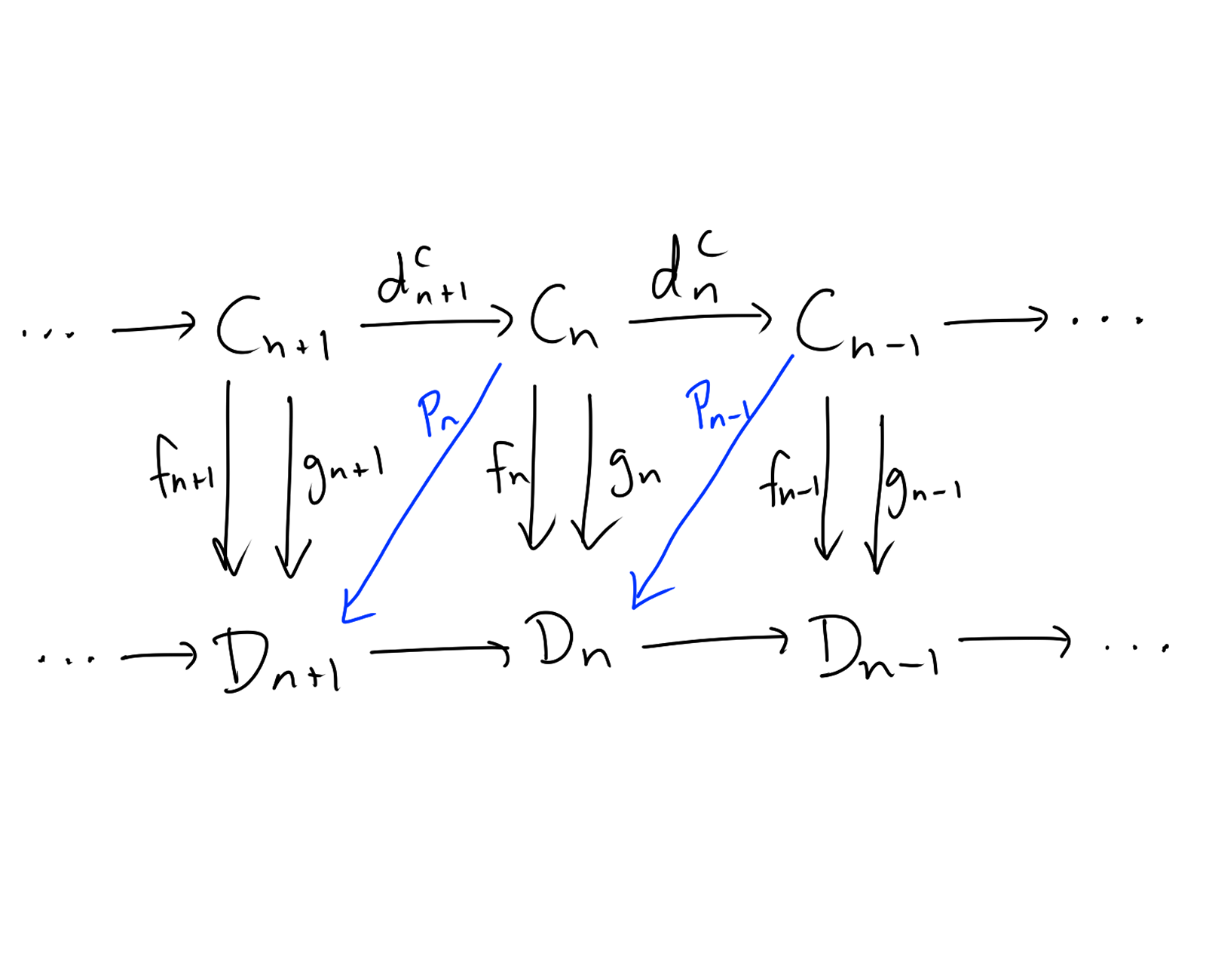
$\textbf{Lemma 2.1.}$ A map $f:X\to Y$ of spaces induces a map $f_\#:C_*(X)\to C_*(Y)$ of chain complexes. $\textit{Proof.}$ Define $f_n:C_n(X) \to C_n(Y)$ by $(\sigma:\Delta^n \to X) \mapsto (f\circ \sigma : \Delta^n \to Y).$ Exercise for you to show that this is indeed a chain map. $\Box$ $\textbf{Lemma 2.2.}$ A map $f_\#:C_*\to D_*$ of chain complexes induces a map $f_*:H_n(C_*)\to H_n(D_*)$ of abelian groups. $\textit{Proof.}$ For $x \in H_n(C_*)$ define $f_n(x) = [f_n(c)]$ where $c \in C_n$ is any representation of $x.$ Exercise for you to show that $f_n(c) \in \ker(d)$, and $f_*$ is a well defined group homomorphism. $\Box$$\textbf{Corollary 2.3.}$ A map $f:X\to Y$ induces a map $f_*:H_n(C_*)\to H_n(D_*).$ Homotopic maps induce the same map on homologyTo show that homotopic maps in topology induce the same map on homology, we introduce a notion of homotopy between chains. A chain homotopy from $f$ to $g$ is a collection of maps $P_n:C_n \to D_{n+1}$ satisfying $d_{n+1}^D\circ P_n + P_{n-1}\circ d_n^C = g_n - f_n.$
\begin{CD}
\ldots @>>> C_{n+1} @>d_{n+1}^C >> C_n @> d_n^C >> C_{n-1} @>>> \ldots \\
@. @V f_{n+1} V g_{n+1} V @V f_{n} V g_{n} V @V f_{n-1} V g_{n-1} V @. \\
\ldots @>>> D_{n+1} @>d_{n+1}^D >> D_n @> d_n^D >> D_{n-1} @>>> \ldots \\
\end{CD}
Exercise: complete the diagram (not commutative). $\textbf{Lemma 2.4.}$ If $f \simeq g : C_* \to D_*$, then $f_* = g_*: H_n(C_*) \to H_n(D_*).$ $\textit{Proof.}$ Exercise by definitions. $\Box$ $\textbf{Theorem 2.5.}$ If $f \simeq g : X \to Y$, then $f_* = g_*: H_n(C_*) \to H_n(D_*).$ $\textit{Proof.}$ Define $P_n(\sigma) = \sum_{i=0}^n (-1)^i F \circ (\sigma \times \id)\mid_{\Delta_i^{n+1}}$ where the union of $\Delta_i^{n+1}$'s form an $n$-simplex for $\Delta^n\times I.$ See Hatcher for the specific prism construction of the $\Delta_i^{n+1}$'s. Perform algebra to verify that this is indeed a homotopy on chain complexes and we are done by Lemma 2.4. $\Box$ Long exact sequence for computing homologyWe will introduce a very useful method for computing homology groups using exact sequences. Firstly, an exact sequence is a sequence
\begin{CD}
\ldots @>>> A_{n+1} @>\alpha_{n+1}>> A_n @>\alpha_n>> A_{n-1} @>>> \ldots
\end{CD}
if $\ker(\alpha_n) = \text{im}(\alpha_{n+1})$ for all $n.$ Some examples of exact sequences are
The reduced homology groups $\tilde{H}_n(X)$ are the homology groups of the augmented chain complex of $C_*(X)$ by appending an extra $C_0(X) \xrightarrow{\epsilon} \mathbb{Z}$ to the end. Note that this gives us $H_n(X) \cong \tilde{H}_n(X)$ for $n>0$ and $H_0(X) \cong \tilde{H}_0(X) \oplus \mathbb{Z}.$ Lastly, say that $(X,A)$ is a good pair if $A$ is nonempty, closed and contained in an open $V$ which deformation retracts to $A.$ Now for the big theorem... $\textbf{Theorem 2.6.}$ Suppose $(X,A)$ is a good pair. Then there exists a long exact sequence
\begin{CD}
\ldots @>>> H_n(A) @>i_*>> H_n(X) @>j_*>> \tilde{H}_n(X/A) @>\partial>> H_{n-1}(A) @>>> \ldots
\end{CD}
Usually, we can take everything else to be reduced homology as well, but $\tilde{H}_n(X/A)$ must always be reduced. $\textit{Proof.}$ We will prove this in three steps with three non trivial theorems.
For the first step, we will prove something more general then apply it to the long exact sequence on relative homology (which we will define after). $\textbf{Theorem 2.7.}$ Suppose we have a short exact sequence $0 \to A_* \xrightarrow{i} B_* \xrightarrow{j} C_* \to 0$ of chain complexes.
\begin{CD}
@. \vdots @. \vdots @. \vdots @. \\
@. @VVV @VVV @VVV @. \\
0 @>>> A_{n+1} @>i_{n+1}>> B_{n+1} @>j_{n+1}>> C_{n+1} @>>> 0 \\
@. @VV d_{n+1}^A V @VV d_{n+1}^B V @VV d_{n+1}^C V @. \\
0 @>>> A_{n} @>i_{n}>> B_{n} @>j_{n}>> C_{n} @>>> 0 \\
@. @VV d_{n}^A V @VV d_{n}^B V @VV d_{n}^C V @. \\
0 @>>> A_{n-1} @>i_{n-1}>> B_{n-1} @>j_{n-1}>> C_{n-1} @>>> 0 \\
@. @VVV @VVV @VVV @. \\
@. \vdots @. \vdots @. \vdots @.
\end{CD}
Then we have a long exact sequence
\begin{CD}
\ldots @>>> H_n(A_*) @>i_*>> H_n(B_*) @>j_*>> H_n(C_*) @>\partial>> H_{n-1}(A_*) @>>> \ldots
\end{CD}
$\textit{Proof.}$ There are two steps to the proof.
Let us start by defining $\partial.$ Let $x \in H_n(C_*)$ and choose a representation $c \in C_n.$ Then $d_n^C(c) = 0.$ Since $j_n$ is surjective, we can choose $b \in B_n$ with $j_n(b) = c.$ By commutativity, we have $j_{n-1}(d_n^B(b))$ $=$ $d_n^C(j_n(b))$ $=$ $d_n^C(c)$ $=$ $0.$ Thus, we have $d_n^B(b) \in \ker(j_{n-1}) = \im(i_{n-1})$ and hence we have $a \in A_{n-1}$ with $i_{n-1}(a) = d_n^B(b).$ We want to let $\p(x) = [a]$ but in order to so we want $a \in \ker(d_{n-1}^A).$ To get this, it suffices to check $i_{n-2}(d_{n-1}^A(a))=0$ by injectivity. But we have $i_{n-2}(d_{n-1}^A(a))$ $=$ $d_{n-1}^B(i_{n-1}(a))$ $=$ $d_{n-1}^B(d_n^B(b))$ $=$ $0.$ Now we checked well definedness of $p.$ We made two choices above with representation of $x$ and choice of $b$ with $j_n(b) = c.$ Now suppose $c' \in C_n$ is a different representation with $c' = c + d_{n+1}^C(c'')$ for some $c'' \in C_{n+1}.$ Now choose $b'' \in B_{n+1}$ with $j_{n+1}(b'') = c''.$ Let $b' = b + d_{n+1}^B(b'').$ Then we have $j_n(b')$ $=$ $j_n(b)+j_n(d_{n+1}^B(b'))$ $=$ $c+d_{n+1}^C(j_{n+1}(b''))$ $=$ $c+d_{n+1}^C(c'')$ $=$ $c'.$ So choose $b'$ mapping to $c'$ and then we get $d_n^B(b')$ $=$ $d_n^B(b + d_{n+1}^B(b''))$ $=$ $d_n^B(b) + d_n^B(d_{n+1}^B(b''))$ $=$ $d_n^B(b).$ This means that we will end up with the same $a.$ Now suppose we choose a different $b'$ mapping to $c.$ Then we have $j_n(b'-b)=c-c=0$ is in $\ker(j_n) = \im(i_n)$ so there exists $a' \in A_n$ with $b' = b + i_n(a').$ Then we end up with $a + d_n^A(a')$ instead of $a$ but this is the same element in homology. $\qed$ 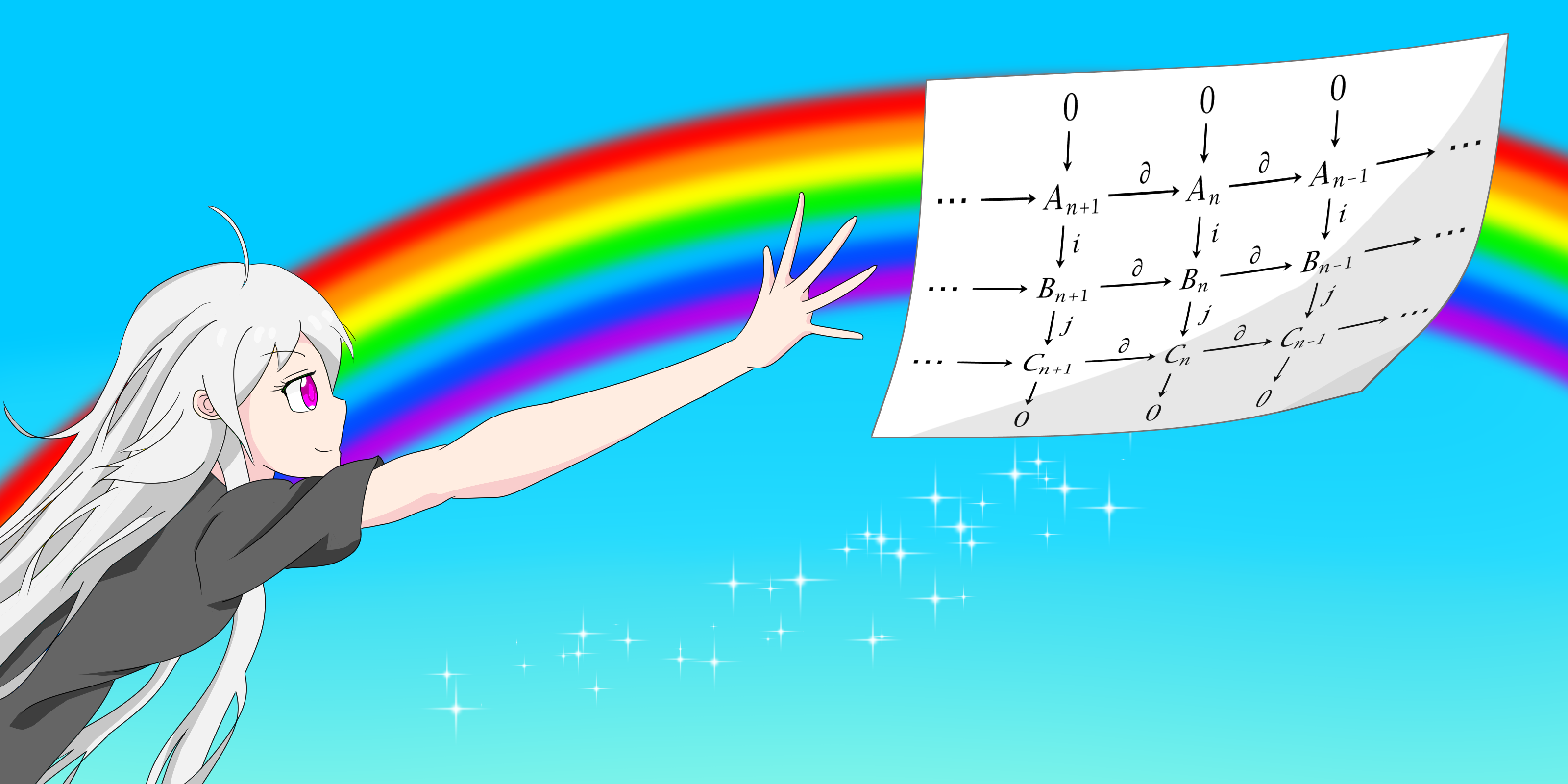
Let us quickly define relative homology. For $A\subset X$, let $C_n(X,A) = C_n(X)/C_n(A)$ and $d_n:C_n(X,A) \to C_{n-1}(X,A)$ defined by $d_n([x]) = [d_n(x)].$ We still have $d_n \circ d_{n+1} = 0$ so we can define $H_n(X,A) = \frac{\ker(d_n)}{\text{im}(d_{n+1})}.$ You should be able to see that the following is a short exact sequence by the obvious maps
\begin{CD}
0 @>>> C_n(A) @> i >> C_n(X) @> j >> C_n(X,A) @>>> 0
\end{CD}
such that we have a long exact sequence on relative homology
\begin{CD}
\ldots @>>> H_n(A) @>i_*>> H_n(X) @>j_*>> H_n(X,A) @>\partial>> H_{n-1}(A) @>>> \ldots
\end{CD}
Again, we can take everything to be reduced homology except $H_n(X,A)$, which is equal to its reduced version. Note that for good point set topology conditions for $B\subset A \subset X$, we also have that a short exact sequence of relative chain complexes
\begin{CD}
0 @>>> C_n(A,B) @>>> C_n(X,B) @>>> C_n(X,A) \to 0
\end{CD}
and long exact sequence of relative homology
\begin{CD}
\ldots @>>> H_n(A,B) @>>> H_n(X,B) @>>> H_n(X,A) @>>> H_{n-1}(A,B) @>>> \ldots
\end{CD}
$\textbf{Theorem 2.8.}$ (Excision) For $Z \subset A \subset X$ with $\bar{Z} \subset \text{int}(A)$,
$$H_n(X/Z,A/Z) \xrightarrow{\cong} H_n(X,A).$$
Equivalently, if $A,B \subset X$ with $\text{int}(A) \cup \text{int}(B) = X$, then
$$H_n(B, A\cap B) \xrightarrow{\cong} H_n(X,A).$$
$\textit{Proof.}$ The proof of this theorem is non trivial and exercise for you is to read the proof in Hatcher. The proof strategy is to show that $\iota: C_*(A+B) \to C_*(X)$ has a deformation retract $\rho:C_*(X) \to C_*(A+B).$ Then $\rho$ induces a chain homotopy equivalence $C_*(X,A) \to C_*(A+B,A)$ and hence an isomorphism on homology. The main idea for the proof is to use barycentric division such that the image of each simplex piece is contained in either $A$ or $B.$ $\Box$ $\textbf{Proposition 2.9.}$ If $(X,A)$ is a good pair, then the quotient map $q:(X,A) \to (X/A , A/A)$ induces an isomorphism $q_*:H_n(X,A) \to H_n(X/A,A/A).$ But since $H_n(X,*) \cong \tilde{H}_n(X)$, we have $$H_n(X,A) \cong \tilde{H}_n(X/A).$$$\textit{Proof.}$ Exercise for you to show that ①,②,③,④,⑤ below are isomorphisms with all the theory covered up to this point for $A\subset V\subset X.$
\begin{CD}
H_n(X,A) @>①>> H_n(X,V) @< ② << H_n(X \setminus A, V \setminus A) \\
@V q_* VV @V q_* VV @V q_* V ③V \\
H_n(X/A,A/A) @>⑤>> H_n(X/A,V/A) @< ④ << H_n(X/A \setminus A/A, V/A \setminus A/A)
\end{CD}
Hint: look at the steps required for the proof of Theorem 2.7. $\Box$ Equivalence between singular and simplicial homologyIf we have a natural transformation $\varphi: h_* \to k_*$ of homology theories which is an isomorphism on spheres, then it is an isomorphism for all $X.$ We will now go on a journey to prove a special case of this: the equivalence between simplicial and singular homology. $\textbf{Lemma 2.10.}$ The identity map $i_n: \Delta^n \to \Delta^n$ is a generator of $H_n(\Delta^n, \partial \Delta^n).$ $\textit{Proof.}$ Induction on $n.$ Define $\Lambda_i^n \subset \partial D^n$ the union of all $[v_0,\ldots,\hat{v_j},\ldots,v_n]$ except for $j=i.$ Then we have
\begin{CD}
H_n(\Delta^n,\partial \Delta^n) @>\cong>> H_{n-1}(\partial \Delta^n, \Lambda_0^n) @<\cong<< H_{n-1}(\Delta^{n-1},\partial \Delta^{n-1}).
\end{CD}
The left isomorphism is given by the mystery map which you can show by a diagram chase sends $[i_n] \in H_n(\Delta^n,\partial\Delta^n)$ to the image of $i_{n-1} \in C_{n-1}(\Delta^{n-1},\partial\Delta^{n-1})$ under the right isomorphism given by excision. $\Box$ $\textbf{Lemma 2.11.}$ (Five Lemma) Suppose the rows of the below diagram are exact and $\alpha,\beta,\delta,\epsilon$ are isomorphisms. Then so is $\gamma.$
\begin{CD}
A @> i >> B @> j >> C @> k >> D @> l >> E \\
@V \alpha VV @V \beta VV @V \gamma VV @V \delta VV @V \epsilon VV \\
A' @> i' >> B' @> j' >> C' @> k' >> D' @> l' >> E' \\
\end{CD}
$\textit{Proof.}$ Easy diagram chase for showing $\gamma$ injective and surjective. $\Box$ $\textbf{Theorem 2.12.}$ (Equivalence between singular and simplicial homology) For any pair $(X,A)$ of $\Delta$-complexes, $$H_n^\Delta(X,A) \xrightarrow{\cong} H_n(X,A).$$$\textit{Proof.}$ First we consider $A = \emptyset.$ Then we prove by induction on skeleton of $X$ (See Hatcher for compactness argument for infinite-dimensional $X$). Let $X^k = k$-skeleton of $X.$ Consider the maps between long exact sequences for simplicial and singular homology.
\begin{CD}
H_{n+1}^\Delta(X^k,X^{k-1}) @>>> H_{n}^\Delta(X^{k-1}) @>>> H_{n}^\Delta(X^k) @>>> H_{n}^\Delta(X^k,X^{k-1}) @>>> H_{n-1}^\Delta(X^{k-1}) \\
@V ① VV @V ② VV @V ③ VV @V ④ VV @V ⑤ VV \\
H_{n+1}(X^k,X^{k-1}) @>>> H_{n}(X^{k-1}) @>>> H_{n}(X^k) @>>> H_{n}(X^k,X^{k-1}) @>>> H_{n-1}(X^{k-1}) \\
\end{CD}
Miscellaneous homology propertiesHere we will list some facts about or applications of homology whose proofs are an exercise for you. Missing definitions are also an exercise for you.
2.2. Computations and ApplicationsHaving explored the built the basic groundwork for homology, we can dive into the wonderful world of computations and applications. We will look at degrees of maps between spheres, cellular homology, Euler characteristic and extensions of homology theory we have built up to this point. DegreeNote that any group homomorphism on $\mathbb{Z}$ is given by multiplication such that the following definition makes sense. The degree of $f:S^n \to S^n$ is the integer $d$ such that $f_*:\tilde{H}_n(S^n) \to \tilde{H}_n(S^n)$ is multiplication by $d.$ Even with this easy definition, we have lots of interesting propositions and theorems.
$\textbf{Proposition 2.13.}$
For a map $f:S^n\to S^n$ we have
$\textit{Proof.}$ We will prove the not so obvious points.
$\textbf{Theorem 2.14.}$ $S^n$ has a nonvanishing vector field if and only if $n$ is odd. A vector field on $S^n$ is a map $v:S^n \to \mathbb{R}^{n+1}$ with $x \bot v(x)$ for all $x \in S^n.$ Nonvanishing means $v(x)\not=0$ such that we can assume $|v(x)|=1.$ $\textit{Proof.}$ Suppose such $v$ exists. Then we have a homotopy $\id\cong A$ given by $f_t(x) = (\cos t)x + (\sin t)v(x)$ for $t \in [0,\pi].$ Then $1 = \deg(\id) = \deg(A) = (-1)^{n+1}.$ If $n$ is odd, we can write $n=2k-1$ and viewing $S^{2k-1}$ as lying in $\mathbb{C}^k$ we define a nonvanishing vector field $v(z_1,\ldots,v_k) = (iz_1,\ldots,iz_k)$ for $i \in \mathbb{C}.$ $\Box$ $\textbf{Theorem 2.15.}$ The only nontrivial group that can act freely on $S^n$ for $n$ even is $\mathbb{Z}/2.$ $\textit{Proof.}$ Exercise for you. Hint: consider defining a map $d:G \to \left\{\pm 1\right\}.$ $\Box$ Let us take a quick detour a define local homology. For $x \in X$, the local homology of $X$ at $x$ is $$H_n(X\mid_x) = H_n(X,X\setminus\left\{x\right\}).$$If $U$ is any open neighbourhood of $x$ we have by excision $$H_n(U\mid_x) = H_n(X\mid_x).$$Before we return to degree, we have the following result using local homology. $\textbf{Theorem 2.16.}$ If nonempty opens $U\subset \mathbb{R}^m$ and $V \subset \mathbb{R}^n$ are homeomorphic, then $m=n.$ $\textit{Proof.}$ A homeomorphism $f:U\to V$ induces an isomorphism $f_*:H_k(U\mid_x)\to H_k(V\mid_y)$ for $y=f(x).$ But we have
$$H_k(U\mid_x) \cong H_k(\mathbb{R}^m,\mathbb{R}^m\setminus\left\{x\right\})\cong
\begin{cases}
\mathbb{Z} & \text{ $k=m$} \\
0 & \text{ else.}
\end{cases}
$$
We have the same result for $H_k(V\mid_y)$ but since the groups are isomorphic, we must have $m=n.$ $\Box$ We will introduce a concept of local degree which will gives us the below theorem helpful for computing global degrees. Let $f:S^n \to S^n$ and suppose $f^{-1}(y)=\left\{x_1,\ldots,x_m\right\}$ is a finite set. Choose disjoint neighbourhoods $U_i$ of $x_i$ and neighbourhood $V$ of $y$ with $f(U_i)\subset V$ for $i=1,\ldots,m.$ Then we can define the map $$f_*:H_n(U_i \mid_{x_i}) \to H_n(V\mid_y).$$But $H_n(U_i\mid_{x_i})$ $=$ $H_n(U_i,U_i\setminus\left\{x_i\right\})$ $\cong$ $H_n(S^n, S^n\setminus\left\{x_i\right\})$ $\cong$ $\mathbb{Z}$ with the first isomorphism given by excision and similarly for $H_n(V\mid_y) \cong \mathbb{Z}.$ Thus, we define local degree of $f$ at $x_i$ as the integer $\deg(f\mid_{x_i})$ such that $f_*$ above is multiplication by this number. We now have a good result. $\textbf{Theorem 2.17.}$ $\deg f = \sum_{i=1}^m \deg f\mid_{x_i}.$ $\textit{Proof.}$ By excision we have
$$H_n(\coprod U_k, \coprod(U_k/\left\{x_k\right\})) \cong H_n(S^n, S^n\setminus\left\{x_1,\ldots,x_m\right\}).$$
But the left hand side is also the homology of a disjoint union of pairs such that
$$H_n(\coprod U_k, \coprod(U_k/\left\{x_k\right\})) \cong \bigoplus H_n( U_k, U_k/\left\{x_k\right\}) \cong \bigoplus \mathbb{Z}.$$
Thus, we have $H_n(S^n, S^n\setminus\left\{x_1,\ldots,x_m\right\})$ $\cong$ $\mathbb{Z}^m.$ Let $e_i$ denote the generator of the $i$-th $\mathbb{Z}.$ Then we have two claims. Claim 1. $f_*(e_i) = \deg f\mid_{x_i}$ Proof of claim 1. Consider the following commutative diagram with all groups isomorphic to $\mathbb{Z}$ except the bottom left which is isomorphic to $\mathbb{Z}^m$ as shown above.
\begin{CD}
H_n(U_i,U_i\setminus\left\{x_i\right\}) @>f_*>> H_n(V, V \setminus\left\{y\right\}) \\
@VVV @VV\cong V\\
H_n(S^n, S^n \setminus\left\{x_1,\ldots,x_m\right\}) @>f_*>> H_n(S^n, S^n\setminus\left\{y\right\})
\end{CD}
At the top, $1$ is sent to $\deg f\mid_{x_i}$, but at the bottom $1$ is sent to $e_i.$ The isomorphism on the right given by excision and commutativity of the diagram gives us $f_*(e_i) = \deg f\mid_{x_i}.$ Claim 2. $j:\tilde{H}_n(S^n)$ $\to$ $H_n(S^n,S^n\setminus\left\{x_1,\ldots,x_m\right\})$ is the diagonal map $1 \mapsto \sum e_i.$ Proof of claim 2. Let $U_k' = U_i \setminus\left\{x_i\right\}$ for $k=i$ and $U_k' = U_k$ otherwise. Then consider the commutative diagram with the bottom two isomorphisms given by excision. 
With claim 2 we get the following commutative diagram.
\begin{CD}
\tilde{H}_n(S^n) @>f_*>> H_n(S^n)\\
@V j VV @V j V\cong V\\
H_n(S^n, S^n \setminus\left\{x_1,\ldots,x_m\right\}) @>f_*>> H_n(S^n, S^n\setminus\left\{y\right\})
\end{CD}
In the diagram we have $(f_* \circ j)(1) = \sum{f_*}(e_i)$ for $1 \in \tilde{H}_n(S^n).$ So by claim 1 and the isomorphism on the right we have $f_*(1) = \sum \deg f\mid_{x_i}.$ $\Box$ Cellular homologyIn this section we will define cellular homology and show it is equivalent to singular and simplicial homology. Cellular homology is good because CW complexes are easier to construct and understand than other complexes. We will start with some homology observations for CW complexes.
$\textbf{Lemma 2.18.}$
Let $X$ be a CW complex. Then we have
$\textit{Proof.}$ We prove for finite dimensional CW complexes. See Hatcher for the harder infinite dimensional case.
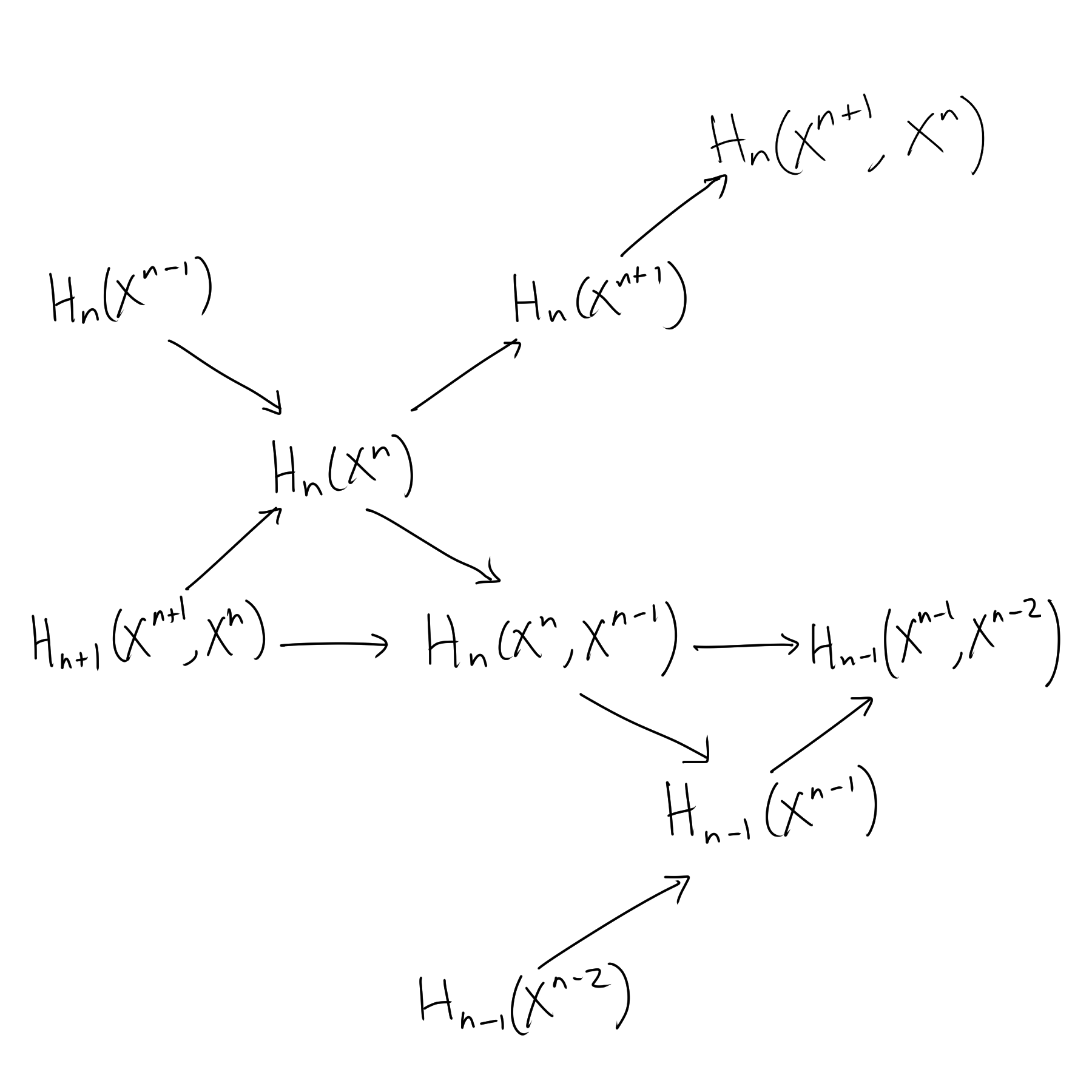
Now we being our journey of defining cellular homology. Define $C_n^{CW}(X) = \mathbb{Z} \left\{ n \text{-cells of $X$} \right\}.$ However, by our lemma above we can identify this with $H_n(X^n, X^{n-1}).$ Then we can define our boundary map $d_n^{CW}$ by the following awesome commutative diagram with exact sequences in the diagonals and the middle row representing our cellular chains. 
So we have $d_n^{CW} = j_{n-1}\circ \partial_n$ and since $d_n^{CW}\circ d_{n+1}^{CW} = 0$ (exercise!), we can define cellular homology in the usual way $$H_n^{CW} = \frac{\ker(d_n^{CW})}{\text{im}(d_{n+1}^{CW})}.$$We now show that cellular homology is equivalent to singular homology, and quote without proof a way to calculate the cellular boundary formula easily from Hatcher. $\textbf{Theorem 2.19.}$ $H_n^{CW}(X) \cong H_n(X).$ $\textit{Proof.}$ Diagram chase on the above diagram to find a group isomorphism $\Phi:H_n^{CW}(X)\to H_n(X).$ $\Box$ $\textbf{Cellular Boundary Formula}$ $d_n(e_\alpha^n) = \sum_\beta d_{\alpha\beta}e_{\beta}^{n-1}$ where $d_{\alpha\beta}$ is the degree of the map $S_\alpha^{n-1} \to X^{n-1} \to S_\beta^{n-1}$ that is the composition of the attaching map of $e_\alpha^n$ with the quotient map collapsing $X^{n-1} - e^{n-1}_\beta$ to a point. Euler characteristicYou have probably heard of the Euler characteristic for the two dimensional case given by $\chi = V - E + F$ with $V,E,F$ denoting number of vertices, edges and faces respectively. We can generalise this definition for finite CW complexes: $$\chi(X) = \sum(-1)^i [\# i\text{-cells in $X$}].$$The reason we consider Euler characteristic only now is because we can use homology to show that it is invariant under choice of CW complex structure of a space. Specifically, we have the following theorem. An application of this fact is left as an exercise for you with the proposition below. $\textbf{Theorem 2.20.}$ $\chi(X) = \sum(-1)^i (\rank(H_i(X))$ $\textit{Proof.}$ Let $C_n = C_n^{CW}(X)$, $Z_n = \ker(d_n^{CW})$, $B_n = \text{im}(d_{n+1}^{CW})$ and $H_n = H_n(X) = Z_n/B_n.$ Then we have two short exact sequences
\begin{CD}
0 @>>> Z_n @>i>> C_n @>d_n>> B_{n-1} @>>> 0 \\
@. @. @. @. @. \\
0 @>>> B_n @>>> Z_n @>>> H_n @>>> 0 \\
\end{CD}
Exercise for you to complete the proof by using the fact that if $0 \to A \to B \to C \to 0$ is a short exact sequence of finitely generated abelian groups then $\text{rank}(B)=\text{rank}(A)+\text{rank}(C).$ $\Box$ $\textbf{Corollary 2.21.}$ $\chi(X)$ is independent of the CW structure on $X.$ $\textbf{Proposition 2.22.}$ (Hatcher 2.2.22) If $X$ a finite CW complex and $p:\tilde{X} \to X$ an $n$-sheeted covering space, then $$\chi(\tilde{X}) = n\chi(X).$$$\textit{Proof.}$ Exercise for you. Hint: think about covering space theorems. $\Box$ Split exact sequencesWe will introduce a general algebra fact that will be useful for computing homologies. A short exact sequence $0 \to A \xrightarrow{i} B \xrightarrow{j} C \to 0$ is split if there is an isomorphism $B \cong A \oplus C$ where the following diagram commutes with the maps below the canonical inclusion and projection. With this definition we have a lemma giving equivalent definitions. 
$\textbf{Lemma 2.23.}$ (Splitting Lemma) Given a short exact sequence $0 \to A \xrightarrow{i} B \xrightarrow{j} C \to 0$, the following are equivalent
$\textit{Proof.}$ Implications $1 \implies 2$ and $1 \implies 3$ are immediate by definitions. For the direction $2 \implies 1$, consider the map $f:B \to A \oplus C, f(b) = (r(b), j(b)).$ Clearly the diagram commutes. To get $f$ injective, suppose $r(b)=0$ and $j(b)=0.$ By exactness, there is some $a$ with $i(a)=b.$ But since $ri = \id$ we get $a=0$ such that $b=0.$ To get $f$ surjective note that $f(i(a)) = (a,0)$ by exactness and $ri = \id$, meaning that we can hit everything in the $A$ component of $A\oplus C$. Moreover, $j$ is surjective, so we can hit anything in the $C$ component, and add some $a$ to get rid of the $r(b)$ leftovers. For $3 \implies 1$, consider the map $g: A \oplus C \to B, g(a,c) = i(a) + s(c).$ Again the diagram commuting is almost immediate. To get $g$ surjective, let $b \in B.$ Then let $c = j(b)$ and note that $js(c) = c$ by assumption. Let $b' = s(c).$ Then $j(b-s(c))=j(b)-js(c)$ $=$ $c-c = 0.$ So by exactness there exists $a$ with $i(a) = b-s(c)$ and hence $i(a) + s(c) = b.$ To get $g$ injective, suppose $i(a)+s(c)=0.$ Then $j$ sends the left hand side to 0 such that by exactness there exists $a'$ with $i(a')=i(a)+s(c)$ and hence $i(a'-a)=s(c)$. Applying $j$ to both sides we get $c=0$ and hence $i(a)=0$ with gives $a=0$ by injectivity of $i.$ $\Box$ An example application of this is if the group at the end of the sequence $C$ is free, then the sequence is split. This is because we can create a map $s:C\to B$ by $s(c) = b$ for some choice of $b \in B$ with $j(b)=c$ by surjectivity which is well defined by assumption that $C$ is free. Another example is if $r: X \to A$ is a retraction, we have $r\circ i =\id$ with $i$ the usual inclusion. Then the induced map $i_*:H_n(A) \to H_n(X)$ is injective since $r_*\circ i_* = \id.$ From the long exact sequence of the pair $(X,A)$ and the splitting lemma, we have the following split sequence
\begin{CD}
0 @>>> H_n(A) @>i_*>> H_n(X) @>j_*>> H_n(X,A) @>>> 0.
\end{CD}
Mayer-Vietoris sequencesRecall that we had a long exact sequence for a good pair $(X,A).$ In fact, we have another very useful long exact sequence known as the Mayer-Vietoris sequence which one could say is the 'van-Kampen theorem' of homology. $\textbf{Mayer-Vietoris sequence.}$ If $\text{int}(A) \cup \text{int}(B) = X$, then we have a long exact sequence on homology
\begin{CD}
\ldots @>>> H_n(A \cap B) @> \Phi >> H_n(A) \oplus H_n(B) @> \Psi >> H_n(X) @> \partial >> H_{n-1}(A\cap B) @>>> \ldots
\end{CD}
$\textit{Proof.}$ With the given assumptions we have a short exact sequence
\begin{CD}
0 @>>> C_*(A\cap B) @> \phi >> C_*(A) \oplus C_*(B) @> \psi >> C_*(A+B) @>>> 0
\end{CD}
The maps are defined by $\phi(x) = (x,-x)$ and $\psi(x,y) = x+y.$ Then by Theorem 2.7 we get the long exact sequence as required. $\textit{Remark.}$ We also have a version of the Mayer-Vietoris sequence for relative homology. Specifically, if $(X,Y) = (A\cup B, C\cup D)$ with $C \subset A, D \subset B$ and good point set conditions, we have
\begin{CD}
\ldots \to H_n(A \cap B, C \cap D) \to H_n(A,C) \oplus H_n(B,D) \to H_n(X,Y) \to H_{n-1}(A\cap B,C\cap D) \to \ldots
\end{CD}
Homology with coefficientsWe can generalise homology to get more 'nice' homology results for certain spaces. Let $G$ be an abelian group. Then we now define chains as free $G$ modules by
$$C_n(X;G) = G\left\{ \sigma: \Delta^n \to X\right\}.$$
Then we can define boundary maps and homology $H_n(X;G)$ in the obvious way. Reduced homology is now induced by adding $C_0(X) \to G$ to the end of the chain complex. Popular choices of $G$ include $\mathbb{Z}/p$, $\mathbb{Z}$ and $\mathbb{Q}.$ In fact, all our homology results up to now still works. A noncomprehensive list of such facts that remain true are as follows.
Now for a quick example of a 'nicer' result, consider $X = \mathbb{R}P^2$ and $G = \mathbb{Z}/2.$ Then our cellular chain complex is $$0 \to G \xrightarrow{d_n} G_n \xrightarrow{d_{n-1}} \ldots \xrightarrow{d_2} G \xrightarrow{d_1} G \to 0,$$with $d_k = 1 + (-1)^k.$ But since $2=0$ in $\mathbb{Z}/2$, we get $$H_k(\mathbb{R} P^n, \mathbb{Z}/2) \cong \begin{cases} \mathbb{Z}/2 & 0\leq k \leq n \\ 0 & \text{else.} \end{cases} $$Moreover, for $G = \mathbb{Z}/p$ with $p$ odd or $G = \mathbb{Q}$ multiplication by 2 is an isomorphism such that $$H_k(\mathbb{R} P^n, G) \cong \begin{cases} G & k=0 \\ G & k=n\text{ is odd} \\ 0 & \text{else.} \end{cases} $$
On top of all the techniques we have so far for computing homology, we have an universal coefficient theorem for computing homology groups with different coefficients. Before we introduce it, let us first look at an interesting exercise from Hatcher. Hatcher 2.2.43 (a) Show that a chain complex of free abelian groups $C_n$ splits as a direct sum of subcomplexes $0\to L_{n+1}\to K_n \to 0$ with at most two nonzero terms. (b) In case the groups $C_n$ are finitely generated, show there is a further splitting into summands $0\to \mathbb{Z} \to 0$ and $0\to \mathbb{Z} \xrightarrow{m} \mathbb{Z} \to 0.$ (c) Deduce that if $X$ is a CW complex with finitely many cells in each dimension, then $H_n(X;G)$ is the direct sum of the following groups:
$\textit{Solution.}$ (a) We have that the short exact sequence $0 \to \ker d_n \xrightarrow{i} C_n \xrightarrow{d_n} \text{im } d_n\to 0$ splits since $\text{im } d_n$ is a subgroup of a free group and hence free. Letting $K_n = \ker d_n$ and $L_n = \text{im } d_n$, this gives us $C_n \cong K_n \oplus L_n.$ Then our chain complex splits as a direct sum of subcomplexes like so
\begin{CD}
\ldots @>>> C_{n+1} @>>> C_n @>>> C_{n-1} @>>> \ldots \\
@. @. \vdots @.\vdots @. @. \\
0 @>>> 0 @>>> L_n @>>> K_{n-1} @>>> 0 \\
@. @. @. @. @. \\
0 @>>> L_{n+1} @>>> K_{n} @>>> 0 @>>> 0 \\
@. @. \vdots @.\vdots @. @. \\
\end{CD}
(b) As the hint in Hatcher suggests, we can represent the injective boundary map $L_{n+1}\cong\mathbb{Z}^p \to K_n\cong\mathbb{Z}^q$ as a $q$ by $p$ matrix $$ \begin{bmatrix} a_{11} & \ldots & a_{1p} \\ \vdots & & \vdots \\ a_{q1} & \ldots & a_{qp} \end{bmatrix} . $$However, an algebra theorem states for a given $A \in M_{qp}(\mathbb{Z})$ there exist $Q \in GL_q(\mathbb{Z}), P \in GL_p(\mathbb{Z})$ such that $Q^{-1}AP$ is diagonal and non zero values on the diagonal $d_1,\ldots,d_k$ such that $d_1 \mid d_2 \mid \ldots \mid d_k.$ The proof idea is an inductive algorithm which gives us a matrix of the following form such that $a_{11}$ divides all elements in the lower right block matrix. $$ \begin{bmatrix} a_{11} & 0 & \ldots & 0 \\ 0 & m_{11} & \ldots & m_{1(p-1)} \\ \vdots & \vdots & & \vdots \\ 0 & m_{(q-1)1} & \ldots & m_{(q-1)(p-1)} \end{bmatrix} . $$This means that by a change of basis matrix for $L_{n+1}$ and $K_n$, we have a linear transformation represented by a diagonal matrix of the form $$ \begin{bmatrix} a_{11} & 0 & \ldots & 0 \\ 0 & a_{22} & \ldots & 0 \\ \vdots & \vdots & & \vdots \\ 0 & 0 & \ldots & a_{pp} \\ 0 & 0 & \ldots & 0 \\ \vdots & \vdots & & \vdots \\ 0 & 0 & \ldots & 0 \\ \end{bmatrix} . $$
The nonzero diagonal entries correspond to the subcomplexes $0\to\mathbb{Z} \xrightarrow{a_{ii}} \mathbb{Z}\to 0$ while the zero rows correspond to the sequences $0 \to \mathbb{Z} \to 0.$
\begin{CD}
\ldots @>>> C_n @>>> C_{n-1} @>>> \ldots \\
@. @.\vdots @. @. \\
0 @>>> L_n @>>> K_{n-1} @>>> 0 \\
@. @.\vdots @. @. \\
0 @>>> 0 @>>> \mathbb{Z} @>>> 0 \\
@. @. @. @. \\
0 @>>> \mathbb{Z} @>m>> \mathbb{Z} @>>> 0 \\
@. @.\vdots @. @. \\
0 @>>> 0 @>>> L_{n-1} @>>> K_n \\
@. @.\vdots @. @. \\
0 @>>> 0 @>>> 0 @>>> \mathbb{Z} \\
@. @. @. @. \\
0 @>>> 0 @>>> \mathbb{Z} @>m>> \mathbb{Z} \\
@. @.\vdots @. @. \\
\end{CD}
Specifically, we get a copy of $G$ corresponding to the $\mathbb{Z}$ in the subcomplex $0\to \mathbb{Z} \to 0$, a copy of $G/mG$ corresponding to the right $\mathbb{Z}$ and a copy of the kernel of $G\xrightarrow{m} G$ corresponding to the left $\mathbb{Z}$ in the subcomplex $0 \to \mathbb{Z} \xrightarrow{m} \mathbb{Z} \to 0.$ $\Box$ Universal coefficient theorem (homology)It is recommended to skip over this for now and return after completing Section 3.1.2 which is about the universal coefficient theorem for cohomology. This is because the proof for the UCT for homology is very similar to that for cohomology so we refer you to the proof there. Now we start with some background definitions. Define a tensor product over $\mathbb{Z}$ on abelian groups $M,N$ by $$M \otimes N = \mathbb{Z}\left\{m\otimes n \mid m \in M, n \in N \right\}/ \sim$$with the equivalence relation generated by the equalities
For $P_\bullet \to M$ a projective resolution, define the $\Tor$ functor by $\Tor_n(M,N) = H_n(P_\bullet \otimes N).$ Similarly to the $\Ext$ functor, we have $\Tor_0(M,N) \cong M \otimes N$ and $\Tor(M,N) = 0$ for $n>1$ so denote $\Tor = \Tor_1.$ With this, we have the following theorem. $\textbf{Theorem 2.24.}$ (Universal coefficient theorem for homology) The following is a short exact sequence. Furthermore it splits but not naturally.
\begin{CD}
0 \to H_i(X) \otimes G \to H_i(X; G) \to \Tor(H_{i-1}(X), G) \to 0.
\end{CD}
$\textit{Proof.}$ Note that $0 \to B_n \to Z_n \to H_n \to 0$ is a projective resolution of $H_n.$ The details of the proof is similar to the universal coefficient theorem for cohomology. $\Box$ 3. Cohomology $H^n(X)$
Cohomology is a bunch of abstract nonsense (haha just joking it's actually very cool!!). Cohomology results from dualisation of chains in homology which result in induced homomorphisms that go the other way. Most of the homology results we have covered up to know also hold in the context of cohomology. The main difference between homology and cohomology is that homology groups are covariant functors, whereas cohomology groups are contravariant. The reason cohomology is better than homology is because it holds more structure as it has a notion of product which arises from this contravariance. In category theory terms, cohomology is a functor $H^*: \mathbf{Top} \to \mathbf{GrRing}$, where $\mathbf{GrRing}$ denotes the category of graded commutative rings with multiplication given by the cup product. You can also read about the topological interpretation of low dimensional cohomology by 'cuts' in Hatcher but we will mainly focus on the algebraic properties of cohomology here. 3.1. Cohomology groupsCohomology definitionsThis section will define cohomology groups from cochains. Fix an abelian group $G$ (later we show that we can take commutative rings).
A map between spaces $f:X\to Y$ induces a map between cochains
\begin{align}
f^\#:C^{n}(Y;G) &\to C^n(X;G) \\
(\phi:C_{n}(Y) \to G) &\mapsto (\phi\circ f_\#: C_n(X) \to G)
\end{align}
which in turn induces a map between cohomology
\begin{align}
f^*:H^{n}(Y;G) &\to H^n(X;G).
\end{align}
As stated earlier, many homology facts hold in cohomology (long exact sequence of a pair, cohomology of $S^n$ and a point, excision, reduced cohomology, relative cohomology etc...). We will not dwelve into this here and refer you to Hatcher. Universal coefficient theorem (cohomology)In this section, we provide a way to calculate cohomology from homology. One might ask why bother with cohomology if we can do this. Firstly, the following theorem does not always provide a way to compute maps in cohomology from maps in homology. Secondly, as mentioned above, cohomology has more structure than homology as we will explore in Section 3.2. At the end of this section we also have a fun exercise to solidify your understanding of the new algebraic terms we will introduce here. Before we state the theorem and proof, let us give some observations, claims and new definitions. If we fix a group $G$ and let $A$ be any group, let $A^* = \Hom(A,G)$ denote its dual. First, note that dualising an exact sequence does not given an exact sequence. A simple example of this is
\begin{CD}
0 @>>> \Z @>2>> \Z @>>> \Z / 2 @>>> 0
\end{CD}
which dualises to the not exact sequence
\begin{CD}
0 @<<< \Z @< 2 << \Z @<<< 0 @<<< 0.
\end{CD}
However, there are certain conditions that make duals of exact sequences exact. $\textbf{Proposition 3.1.}$ If $0\to A\to B \to C \to 0$ is a split exact sequence, then it dualises to an split exact sequence $0 \leftarrow A^* \leftarrow B^* \leftarrow C^* \leftarrow 0$ with $B^* \cong A^* \oplus C^*.$ $\textbf{Proposition 3.2.}$ If $C$ is free, then $0 \to A \xto{i} B \xto{p} C \to 0$ splits. $\textit{Proof.}$ If $C = \Z\set{x_i}$, since $p$ is surjective, we can choose $y_i \in B$ with $p(y_i) = x_i.$ Define the map $s:C\to B$ by $s(\sum n_ix_i) = \sum n_iy_i.$ $\Box$ $\textbf{Proposition 3.3.}$ The dual of the exact sequence $A \xto{i} E \xto{j} B \to 0$ given by $\Hom(A,N) \to \Hom(B,N) \xto{j^*} \Hom(E,N) \xto{i^*}$ is exact. $\textit{Proof.}$ For $j^*$ injective, suppose $j^*(\phi) = 0.$ Then $\phi \circ j = 0$ and hence for all $x \in E$ $\phi(j(x)) = 0.$ But $j$ is surjective so for all $y \in B, \phi(y) = 0$ and hence $\phi=0.$ The fact that $i^* \circ j^* = 0$ is immediate by dualising so $\im(j^*) \subset \ker(i^*).$ For $\ker(i^*) \subset \im(j^*)$, suppose $i^*(\phi) = \phi\circ i = 0.$ Then for $\psi$ defined by $\psi([e]) = \phi(e)$, we have $\phi = j^* (\psi).$ $\qed$ We will introduce a generalisation of the idea of free groups to rings. Note that you can substitute the word "free" for "projective" for this section but we will provide definitions for the former for sake of completeness. This is because as we will see from the definition that a $\Z$-module is an abelian group and free abelian groups are projective with proof idea similar to that of the previous proposition. 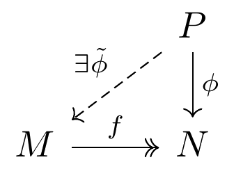
Let $R$ be a ring. An $R$-module $P$ is projective if for all groups $M,N$ if there is a map $\phi:P \to N$ and a surjective map $f:M \to N$, there exists (not necessarily unique) a map $\tilde{\phi}: P \to M$ with $\phi = f \circ \tilde{\phi}.$ A projective resolution of $M$ is the exact sequence below with each $P_i$ projective
\begin{CD}
\ldots @>{d_3}>> P_2 @>{d_2}>> P_1 @>{d_1}>> P_0 @>{\e}>> M @>>> 0.
\end{CD}
Let $P_\dot = \ldots \xto{d_3} P_2 \xto{d_2} P_1 \xto{d_1} P_0 \to 0.$ Then $H_0(P_\dot) = M$ and trivial homology otherwise. Then we can view $P_\dot$ as a "replacement" chain complex for $M$ thought as a chain complex as follows.
\begin{CD}
\ldots @>{d_3}>> P_2 @>{d_2}>> P_1 @>{d_1}>> P_0 @>>> 0 \\
@. @VV 0 V @VV 0 V @VV \e V \\
\ldots @>>> 0 @>>> 0 @>>> M @>>> 0.
\end{CD}
This diagram commutes and induces an isomorphism on homology by exactness. Specifically, by the first isomorphism theorem, $M \cong P_0/\ker(\e) \cong P_0/\im(d_1).$ Now we provide a lemma which will be useful for building up necessary theorem for the universal coefficient theorem. $\textbf{Lemma 3.4.}$ Given $f: M \to N$ and projective resolutions $P_\dot \to M$ and $Q_\dot \to N$, the diagram can be extended to a chain map. Moreover, any two such chain maps are chain homotopic. 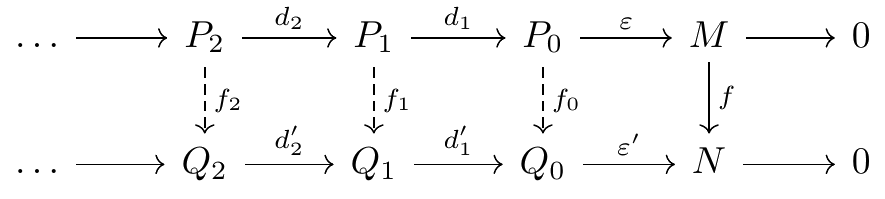
$\textit{Proof.}$ To define $f_0$, use that $P_0$ is projective. To define $f_1$, note that $\e \circ d_1 = 0$$\implies$$f\circ\e\circ d_1 =0$$\implies$$\e'\circ f_0\circ d_1=0$ such that $\im(f_0\circ d_1) \subset \ker(e') = \im(d_1').$ Then use that $P_1$ is projective and continue in this fashion. To get chain homotopy, suppose we have two such chain maps $f_\dot, g_\dot:P_\dot \to Q_\dot.$ Define a chain homotopy $F_n:Pn \to Q_{n+1}$ inductively such that $d_{n+1}' \circ F_n + F_{n-1} \circ d_n = f_n - g_n.$ $\Box$ 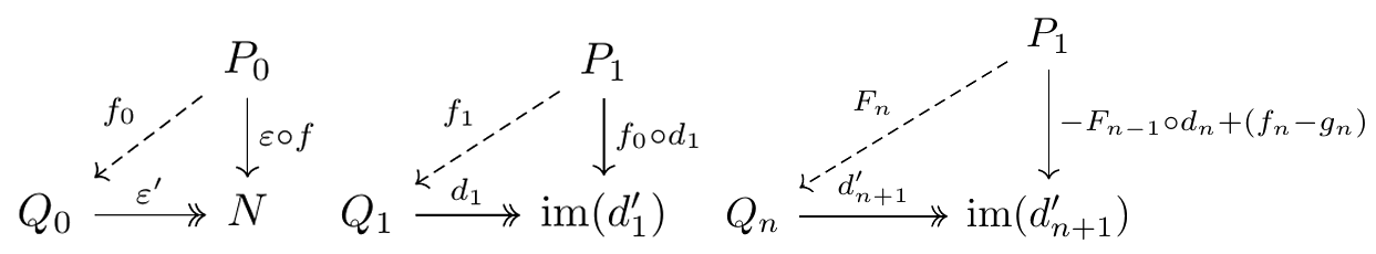
Define $\Ext^n(M,N)$ to be the $n$th cohomology group of the cochain complex $\Hom(P_\dot,N)$ for a projective resolution $P_\dot$ of $M.$ Here, $\Ext$ stands for isomorphism classes of extensions $0\to N\to E \to M\to 0$ but this will not matter for the content of this class. We have the following useful result. $\textbf{Lemma 3.5.}$ $\Ext$ is independent of choice of $P_\dot.$ $\textit{Proof.}$ Suppose we use $P_\dot \to M$ and $Q_\dot \to M.$ Then by the previous lemma, $\id: M \to M$ induces a chain map $\Hom(Q_\dot, N) \to \Hom(P_\dot,N)$ and a map from one definition of $\Ext^n$ to the other. Reversing the roles of $P_\dot$ and $Q_\dot$ gives a map the other way for our isomorphism. $\qed$
$\textbf{Lemma 3.6.}$
$\Ext$ can be computed as follows. The second point is a special case for $\Z$-modules.
$\textit{Proof.}$ The first point is a result from Proposition 2.27. For any abelian group $M$, we have a projective resolution $0 \to \ker(\e) = P_1 \to P_0 \xto{\e} M=0.$ $\qed$ Because of this, write $\Ext(M,N)$ for $\Ext^1(M,N)$ when dealing with abelian groups. Now we have all the necessary theory to state and prove the universal coefficient theorem for cohomology. $\textbf{Theorem 3.7.}$ (Universal coefficient theorem for cohomology) If $C_*$ is a chain complex of free abelian groups, then the following is a short exact sequence. Furthermore, it splits but not naturally.
\begin{CD}
0 @>>> \Ext(H_{n-1}(C_*), G) @>>> H^n(C_*;G) @>>> \Hom(H_n(C_*), G) @>>> 0.
\end{CD}
$\textit{Proof.}$ Let use define some groups as follows.
\begin{CD}
0 @>>> Z_{n+1} @>i>> C_{n+1} @>d_{n+1}>> B_n @>>> 0.\\
@. @VV0V @VVd_{n+1}V @VV0V @.\\
0 @>>> Z_{n} @>i>> C_{n} @>d_{n}>> B_{n-1} @>>> 0.
\end{CD}
Since $B_n$ is free we dualise and again get a short exact sequence.
\begin{CD}
0 @<<< Z_{n-1}^* @<<< C_{n-1}^* @<<< B_n^* @<<< 0.\\
@. @AA 0 A @AA d_{n+1}A @AA 0 A @.\\
0 @<<< Z_{n}^* @<<< C_{n}^* @<<< B_{n-1}^* @>>> 0.
\end{CD}
Then we get a long exact sequence on cohomology groups
\begin{CD}
\ldots @>>> Z_{n-1}^* @>i_{n-1}^*>> B_{n-1}^* @>>> H^n @>>> Z_n^* @>i_n^*>> B_n^* @>>> \ldots
\end{CD}
Then taking certain subgroups of the above long exact sequence, we have short exact sequences of the form
\begin{CD}
0 @>>> \coker(i_{n-1}^*) @>>> H^n(C_*;G) @>>> \ker(i_n^*) @>>> 0.
\end{CD}
There are two steps left here: to show that the cokernel and kernel are the groups in the theorem, and to show that the sequence is split. Now note that $H_n = Z_n/B_n$ so the following is a projective resolution of $H_n$
\begin{CD}
0 @>>> B_n @>i_n>> Z^n @>j_n>> H_n @>>> 0.
\end{CD}
Then by definition of $\Ext^n$ for this projective resolution (cochain complex is given by $0 \to Z_n^* \xto{i_n^*} B_n^* \to 0$) and the previous lemma, we have $\coker(i_{n-1}^*) \cong \Ext(H_{n-1},G)$ and $\ker(i_n^*) \cong \Ext^0(H_n,G) \cong \Hom(H_n, G).$ To see that the sequence splits, we will give a splitting by a map from $\ker(i_n^*)$ to cohomology as follows. We have a splitting by choosing the projection $(p:C_n \to Z_n) \in C_n^*$ which makes $0 \to Z_n \to C_n \to B_{n-1}$ split. Specifically, given $(\phi:Z_n \to G) \in \ker(i_n^*)$ we have $p^*(\phi)$ $=$ $(\phi\circ p:C_n \to G) \in C_n^*.$ Then $d^{n+1}(\phi \circ p)$ $=$ $\phi\circ p\circ d_{n+1}$ $= 0$ since $\phi \in \ker(i_n^*)$ such that $[\phi\circ p ] \in H^n(C_*, G).$ $\qed$ Here are some more useful ways to compute $\Ext$ and hence cohomology with the universal coefficient theorem. $\textbf{Lemma 3.8.}$ For finitely generated $M$ we have
$\textit{Proof.}$
Horseshoe mathematicsNow let's get to the fun exercise we promised. Here we will be talking about horseshoes (not this one!) which will give a long exact sequence for $\Ext.$ What nonsense could I possibly mean? Let's find out. $\textbf{Lemma 3.9.}$ (Horseshoe Lemma) Suppose we have a diagram
\begin{CD}
@. @. @. 0 \\
@. @. @. @VVV \\
\ldots @>>> P_1 @>>> P_0 @>\e_A>> A @>>> 0 \\
@. @. @. @VViV \\
@. @. @. B \\
@. @. @. @VVjV \\
\ldots @>>> Q_1 @>>> Q_0 @>\e_C>> C @>>> 0 \\
@. @. @. @VVV \\
@. @. @. 0 \\
\end{CD}
where the rows are projective resolutions of $A$ and $C$ and $0\to A\to B\to C\to 0$ is exact. Then there is a projective resolution $R_\dot$ of $B$ and maps making $0\to P \to R \to Q \to 0$ a short exact sequence of chain complexes. $\textit{Proof.}$ Let $R_\dot = P_\dot \oplus Q_\dot$ with the obvious maps $i$ and $pr$ (inclusion and projection) that make $0 \to P \to R \to Q \to 0$ exact and split. Then define $\e_B:P_0 \oplus Q_0 \to B$ by $\e_B(p,q) = i(e_A(p)) + s(q)$ where $s$ is the lift from $Q_0$ to $B$ by $Q_0$ projective. It is almost immediate that the diagram commutes with this definition. To get $\e_B$ surjective, let $b \in B$ and pick $q \in Q_0$ with $e_C(q) = j(b).$ Consider $b' = b-s(q).$ Then $j(b')$ $=$ $j(b) - j(s(q))$ $=$ $q(b) - q(b)$ $=$ $0.$ So there exists $a \in A$ with $i(a) = b'.$ Pick $p \in P_0$ with $\e_A(p)=a.$ Then $\e_B(p,q) = b.$ Continue similarly in this way for the rest of $R_\dot.$ $\qed$ $\textbf{Corollary 3.10.}$ If $0\to A\to B\to C\to 0$ is exact and $P_\dot$ and $Q_\dot$ are projective resolutions of $A$ and $C$ respectively, then we have a long exact sequence
\begin{CD}
\ldots @>>> \Ext^n(C,G) @>>> \Ext^n(B,G) @>>> \Ext^n(A,G) @>>> \Ext^{n+1}(C,G) @>>> \ldots
\end{CD}
$\textit{Proof.}$ Exercise by definitions. $\qed$ 3.2. Cup productAs promised, this section will show how to induce a graded ring structure of cohomology groups. Specifically, we will introduce a product between cohomology groups known as the cup product $\smile : H^i \times H^j \to H^{i+j}.$ There are two possible ways to define such a cup product but both are equivalent, one using singular cochains and another using cellular cochains. The cup product is useful because it makes cohomology a more powerful invariant, as some non homotopic equivalent spaces which have isomorphic homology may have different cohomology rings. Do note however, we are dwelving into very abstract land and will be skipping most of the proofs and refering you to Hatcher. Graded groups and ringsBefore we move on to defining the cup product let us define what a graded object is. A graded abelian group $A$ is $A = \oplus_{n \in \Z} A_n$ and we say $x \in A_n$ is in degree $n.$ An example of a graded abelian group is the homology of any space. Usually, it is fine to just call graded abelian groups just "groups with indexing" since there is no interaction between different group components. A graded ring is a graded abelian group $A = \bigoplus A_n$ with a multiplication map $A \times A \to A$ which makes $A$ into a ring. If $a \in A_k,$ $b \in A_l,$ then we required $ab \in A_{k+l}.$ Moreover, the multiplicative identity must be $1 \in A_0.$ An example of a graded ring is a polynomial ring $A \cong R[x]$ where degree of an element here is equal to degree in the polynomial sense. We will see that the cup product makes cohomology into a graded ring. Cup product definition using singular cochainsLet us start with one way of defining the cup product. Similarly to how we first defined homology with singular homology and then cellular homology, this first definition we give is a bit less intuitive but is easier to prove some fundamental cup product properties. Given a cochain $C^*(X;R),$ define the cup product on cochains as follows. For $\phi \in C^k(X;R),$ $\psi \in C^l(X;R),$ $\phi\smile\psi \in C^{k+1}(X;R)$ is given by
$$(\phi \smile \psi)(\s) = \phi(\s\mid_{[v_0,\ldots,v_k]}) \cdot \psi(\s\mid_{[v_k,\ldots,v_{k+1}]}).$$
We have the following lemma for cobundary maps and cup products which will help show that the cup product on cochains induces a well defined cup product on cohomology. $\textbf{Lemma 3.11.}$ $d^{k+l+1}(\phi \smile \psi)$ $=$ $d^{k+1}(\phi) \smile \psi + (-1)^k \psi \smile d^{l+1}(\psi).$ $\textit{Proof.}$ This follows by definitions and some algebra. For $\s : \D^{k+l+1} \to X,$ we have
\begin{align}
d^{k+l+1}(\phi\smile\psi)(\s) &= (\phi\smile\psi)(d_{k+l+1}(\s)) \\
&= (\phi\smile\psi)\lr{\sum_{i=0}^{k+l+1} (-1)^i \s\mid_{[v_0,\ldots,\hat{v_i},\ldots,v_{k+l+1}]}} \\
&= \sum_{i=0}^k (-1)^i \phi(\s\mid_{[v_0,\ldots,\hat{v_i},\ldots,v_{k+1}]}) \cdot \psi(\s\mid_{[v_{k+1},\ldots,v_{k+l+1}]}) \\
&\hspace{3em} +\sum_{i=k+1}^{k+l+1} (-1)^i \phi(\s\mid_{[v_0,\ldots,v_{k+1}]}) \cdot \psi(\s\mid_{[v_{k+1},\ldots,\hat{v_i},\ldots,v_{k+l+1}]}) \\
d^{k+1}(\phi) \smile \psi + (-1)^k \psi \smile d^{l+1}(\psi) &=
\sum_{i=0}^{k+1} (-1)^i \phi(\s\mid_{[v_0,\ldots,\hat{v_i},\ldots,v_{k+1}]}) \cdot \psi(\s\mid_{[v_{k+1},\ldots,v_{k+l+1}]}) \\
&\hspace{3em} +\sum_{i=k+1}^{k+l+1} (-1)^i \phi(\s\mid_{[v_0,\ldots,\hat{v_i},\ldots,v_{k+1}]}) \cdot \psi(\s\mid_{[v_{k+1},\ldots,v_{k+l+1}]}).
\end{align}
Now the $i=k+1$ term of the first sum cancels with the $i=k$ term of the second sum for the right hand side $d^{k+1}(\phi) \smile \psi$ $+$ $(-1)^k \psi \smile d^{l+1}(\psi)$ such that we are left with $d^{k+l+1}(\phi\smile\psi).$ $\qed$ Note that $\smile$ is bilinear so this gives $\smile:C^k(X;R) \otimes_{R} C^l(X;R) \to C^{k+l}(X;R).$ Now we show that this induces a cup product on cohomology. $\textbf{Lemma 3.12.}$ The cup product on cochains induces a well defined cup product on cohomology. $\textit{Proof.}$ For $x\in H^k(X;R)$ and $y \in H^l(X;R)$ choose representatives $\phi$ and $\psi$ and define $x\smile y = [\phi \smile \psi].$ Then $d^{k+1}(\phi)=0,$ $d^{l+1}(\psi)=0,$ so by the lemma we have $d^{k+l+1}(\phi\smile \psi) = 0.$ Hence $\phi \smile \psi$ represents a cohomology class. To get well definedness suppose $\phi'$ is another representation of $x.$ Then $\phi' = \phi + d^k(\xi)$ and again by the previous lemma $\phi' \smile \psi$ $=$ $\phi \smile \psi + d^{k+l}(\xi \smile \psi)$ such that $[\phi' \smile \psi] = [\phi \smile \psi].$ The case for different representation of $y$ is similar. $\qed$ Let us skip example computations and refer to Hatcher for those. Instead we will show commutativity between induced cohomology maps and cup product, and introduce a notion of graded commutativity. $\textbf{Lemma 3.13.}$ For $f:X \to Y,$ $f^*:H^*(Y;R) \to H^*(X;R)$ satisfies $f^*(\a \smile \b) = f^*(\a) \smile f^*(\b).$ $\textit{Proof.}$ This follows because $f^\# (\phi \smile \psi) = f^\# (\phi) \smile f^\#(\psi)$ for $\phi \in C^k(Y;R),$ $\psi \in C^l(Y;R)$ cochains, both are given by $C_{k+1}(X) \to R,$ $\s \mapsto \phi(f\circ \s\mid_{[v_0,\ldots,v_k]})\cdot \psi(f\circ\s\mid_{[v_k,\ldots,v_{k+1}]}).$ $\qed$ $\textbf{Theorem 3.14.}$ If $R$ is commutative, then $H^*(X;R)$ is (graded) commutative. This means for $\a \in H^i(X;R)$ and $\b \in H^j(X;R),$ we have $\a\b = (-1)^{ij} \b\a.$ $\textit{Proof sketch.}$ For $\s:\D^n \to X,$ let $\bar{\s}:\D^n \to X$ be the $n$-simplex obtained by precomposing with reversing the order of vertices $\D^n \to \D^n,$ $v_i \mapsto v_{n-i}.$ Claim that $\r_n:C_n(X) \to C_n(X),$ $\s \mapsto \e_n\bar{\s},$ $\e_n = (-1)^{n(n+1)/2}$ is a chain map chain homotopic to $\id.$ The proof idea for this claim is that we swap two vertices $n$ choose $2$ times while reversing the order of vertices. For $\phi \in C^k(X;R)$ and $\psi \in C^l(X;R),$ we have
\begin{align}
(\r^*\phi \smile \r^*\psi)(\s) &= \e_k\e_l\phi(\s\mid_{[v_k,\ldots,v_0]})\cdot\psi(\s\mid_{[v_{k+l},\ldots,v_k]}) \\
\r^*(\psi\smile\phi)(\s) &= \e_{k+l}\psi(\s\mid_{[v_{k+l},\ldots,v_k]})\cdot\phi(\s\mid_{[v_k,\ldots,v_0]}).
\end{align}
So since $\r$ is chain homotopic to the identity, we have $[\r^*\phi \smile \r^*\psi] = [\phi\smile\psi]$ and $[\r^*(\psi\smile\phi)] = [\psi\smile\phi].$ They differ by sign $\e_k\e_l\e_{k+l}$ which equals $-1$ if both $k$ and $l$ are odd and $1$ otherwise. $\qed$ $\textbf{Corollary 3.15.}$ If $\a \in H^n(X;R)$ with $n$ odd, then $\a \smile \a = -(\a \smile \a)$ such that $2\a^2 = 0.$
$\textbf{Theorem 3.16.}$ The following are graded ring isomorphisms.
$\textit{Proof.}$ See Hatcher, or see Section 3.2 on Poincaré duality. $\qed$ Cup product definition using cellular cochainsNow let us define cup product using cellular cochains by first defining a cross product
$$H^k(X;R) \times H^l(Y;R) \to H^{k+l}(X\times Y;R)$$
which also gives us a product on homology
$$H_k(X;R) \times H_l(Y;R) \to H_{k+l}(X\times Y;R).$$
One way we could do it is by $(\a,\b) \mapsto p_1^*(\a) \smile p_2^*$ with $p_1: X\times Y \to X$ and $p_2: X\times Y \to Y$ projections, but this is boring and does not work for homology. Recall that if $X$ and $Y$ are CW complexes, $X\times Y$ inherits a CW structure with one $(k+l)$-cell for each pair $(e_\a^k,e_\b^l).$ The attaching map for $e_\z^k \times e_\b^l$ is
$$\p(D^{k+l}) = \p D^k \times D^l \bigcup_{\p D^k \times \p D^l} D^k \times \p D^l \;\xto{\phi_\a \times \Phi_\b \;\cup\; \Phi_\a \times \phi_\b}\; (X \times Y)^{k+l-1}.$$
The upshot of this is we have
\begin{align}
C_n^{CW}(X\times Y; R) &\cong \bigoplus_{k+l=n} C_k^{CW}(X;R) \otimes_R C_l^{CW}(Y;R) \\
d_n(x\otimes y) &= d_k(x) \otimes y + (-1)^k x \otimes d_l(y)
\end{align}
for $x \in C_k(X;R), y \in C_l(Y;R).$ Then we have maps
\begin{align}
C_k^{CW} (X;R) \otimes_R C_l^{CW}(Y;R) &\to C_{k+l}^{CW}(X \times Y; R) \\
\implies H_k (X;R) \otimes_R H_l(Y;R) &\to H_{k+l}(X \times Y; R) \\
(\a,\b) &\mapsto \a \times \b.
\end{align}
If $[\phi] \in H^k(X;R)$ and $[\psi] \in H^l(Y;R),$ then we have
\begin{align}
\phi\times\psi(e_\a^p \times e_\b^q) =
\begin{cases}
\phi(e_\a^p) \cdot \psi(e_\b^q) & p=k,q=l \\
0 & \text{else.}
\end{cases}
\end{align}
This defines $[\phi \times \psi] \in H^{k+l}(X\times Y;R)$ and hence we can define the cup product on $H^*(X;R)$ cohomology by composition of the cross product and the diagonal map $\D(x) = (x,x).$ Note the following argument does not work for homology as the arrows go the wrong way.
$$H^k(X;R) \otimes_R H^l(X;R) \to H^{k+l}(X \times X; R) \xto{\D^*} H^{k+l}(X;R).$$
A Künneth formulaIn this section we will state a Künneth formula without proof and instead refer you to Hatcher. This is useful for computing homology groups and cohomology rings of products of spaces. $\textbf{Theorem 3.17.}$ Suppose either that $H^k(X;R)$ or $H^k(Y;R)$ is a finitely generated projective $R$-module for all $k.$ Then the cross product
$$H^*(X;R) \otimes_R H^*(Y;R) \to H^*(X\times Y;R)$$
is an isomorphism of graded rings where the ring structure of the left hand side is given by
$$(x\otimes y)\cdot(x'\otimes y') = (-1)^{|y||x'|}(xx'\otimes yy').$$
With similar conditions we have a version for homology, an isomorphism of graded abelian group
$$H_*(X;R) \otimes_R H_*(Y;R) \to H_*(X\times Y;R).$$
Furthermore, if we have $F$-coefficients for a field $F,$ then
\begin{align}
H^n(X;F) &\cong \Hom_F(H_n(X;F),F) \\
H^n(X\times Y;F) &\cong \bigoplus_{k+l=n} H^k(X;F) \otimes_F H^l(Y;F).
\end{align}
An example of this is the cohomology of the product of infinite dimensional real and complex projective spaces.
\begin{align}
&H^*((\RP^\infty)^n;\Z/2) \cong \Z/2[x_1,\ldots,x_n], \quad |x_i| = 1 \\
&H^*((\CP^\infty)^n;R) \cong R[x_1,\ldots,x_n], \quad |x_i| = 2.
\end{align}
3.3. Poincaré DualityThe reasons for why manifolds are good are manifold. Although we usually focus on global topological properties of spaces in algebraic topology, in this section we will focus on manifolds, whose main feature is their local topology. Specifically, we will see an interesting symmetry between the homology and cohomology groups of manifolds. ManifoldsAn n-manifold is a Hausdorff space $M$ which is locally homeomorphic to $\R^n$ and in the context of manifolds, $M$ is called closed if it is compact. One can consider manifolds with boundary where a neighbourhood is allowed to look like $[0,\infty) \times \R^{n-1}.$ An $\e$-ball in $\R^n$ is homemorphic to $\R^n,$ so asking for neighbourhoods homemorphic to $\R^n$ or homemorphic to an open set in $\R^n$ comes out to the same thing. An example of a closed $n$-manifold is $S^n$ with open cover given by $U_1 = S^n \setminus \set{N}$ and $U_2 = S^n \setminus \set{S}$ with $N$ and $S$ the poles. We also have that $M_g$ and $N_g$ are closed $2$-manifolds. $\RP^n$ is also a closed $n$-manifold with open cover $U_i$ $=$ $\set{[x_0,\ldots,x_n]\mid x_i \not=0}$ $\cong$ $\R^n$ with homeomorphism given by $[x_0,\ldots,x_n]$ $\to$ $\lr{\frac {x_0}{x_i},\ldots,\frac {x_{i+1}}{x_i},\frac {x_{i-1}}{x_i},\ldots \frac {x_n}{x_i} }.$ $\CP^n$ is also a $2n$-manifold. $\R^n$ is a manifold but not a closed manifold. OrientationsNote that for $M$ an $n$-manifold, for any $x \in M$ we have by excision $H_n(M,M\setminus\set{x})$ $\cong$ $H_n(\R^n,\R^n\setminus\set{x})$ $\cong$ $\Z.$ Then a local orientation of $M$ at $x$ is a choice of generator $\m_x$ of $H_n(M,M\setminus\set{x}).$ An orientation of $M$ is a local orientation of $M$ at $x$ for all $x \in M$ which are compatible: If $B \in \R^n$ is a ball of finite radius and $x,y\in B,$ then
\begin{align}
H_n(M,M\setminus\set{x}) \xfrom{\cong} H_n(M&,M\setminus B) \xto{\cong} H_n(M,M\setminus\set{y}) \\
\m_x \from &\m_B \mapsto \m_y.
\end{align}
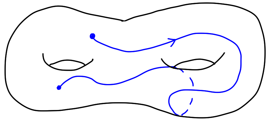
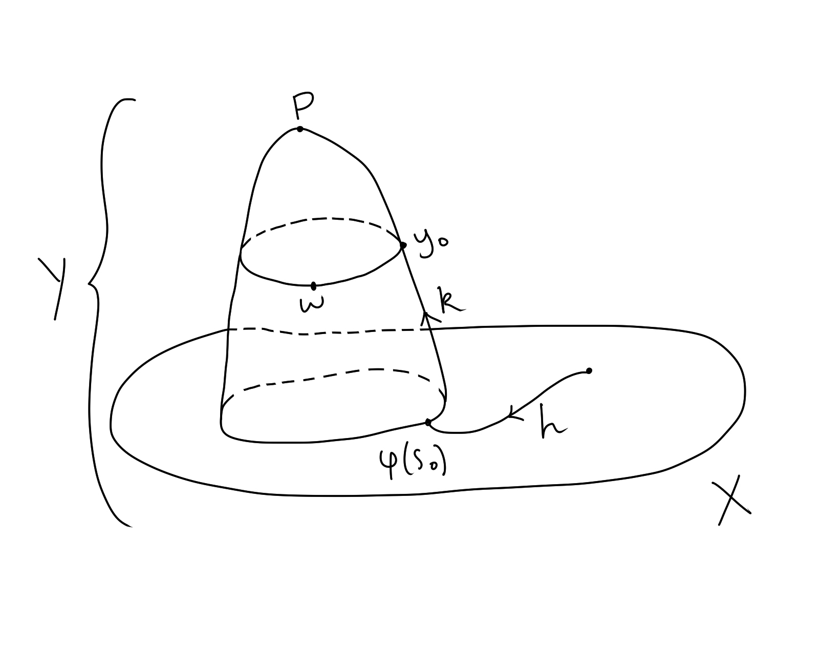
Given a path $\g$ from $x$ to $y$ in $M$ and a local orientation $\m_x$ at $x,$ can use $\g$ to transport $\m_x$ to a local orientation $\m_y$ at $y.$
$\textbf{Lemma 3.18.}$ If $\g_1 \simeq \g_2$ as paths from $x$ to $y,$ then transporting $\m_x$ to an orientation at $y$ using $\g_1$ or $\g_2$ gives the same $\m_y.$
For $M$ path connected, it suffices to consider which loop at $x_0$ preserve and reverse the orientation. This is measured by a group homomorphism
\begin{align}
\pi_1(M,x_0) &\to \set{\pm 1} \cong \Z/2 \\
[\g] &\mapsto
\begin{cases}
+1 & \text{if $\g$ preserves orientation} \\
-1 & \text{if $\g$ reverses orientation.}
\end{cases}
\end{align}
$\textbf{Lemma 3.19.}$ Suppose $X$ is path connected. Then $\Hom(\pi_1(X,x_0),\Z/2)$ $\cong$ $H^1(X,\Z/2).$ $\textit{Proof.}$ Exercise. Note this is true for any abelian group $G$ in place of $\Z/2.$ \qed $\textbf{Corollary 3.20.}$ If $H^1(M,\Z/2) = 0,$ then $M$ is orientable.
The converse of this statement is not true. For example, $H^1(\RP^2, \Z/2)$ $\cong$ $H^1(\RP^3,\Z/2)$ $\cong$ $\Z/2$ and $\RP^2$ is not orientable but $\RP^3$ is orientable. We can generalise. An $R$-orientation of $M$ is a compatible choice of $\m_x \in H(M,M\setminus\set{x};R)$ for all $x \in M.$ Note that any $n$-manifold is $\Z/2$ orientable.
$\textbf{Theorem 3.21.}$
Let $M$ be a closed connected $n$-manifold.
$\textit{Proof.}$ In case 1., a generator of $H_n(M;R)$ is called a fundamental class and is denoted by $[M].$ 3. is clear by putting a CW complex structure on $M.$ Now write $H_n(M/A)$ for $H_n(M,M/A).$ We have the following claim. Let $A,B \subset M$ be compact and suppose we have $\m_A \in H_n(M\setminus A)$ and $\m_B \in H_n(M\setminus B)$ which restricts to a local orientation at $a$ for all $x \in A$ or $x \in B.$ Also suppose these local orientations agree on $A\cap B.$ Then there exists $\m_{A\cup B} \in H_n(M\mid A\cup B)$ which restricts to a local orientation at $x$ for all $x \in A \cup B.$ The proof the claim is given by the Mayer-Vietoris sequence.
$$\ldots \to H_{n+1}(M \setminus A \cap B) \to H_n(M\setminus A\cup B) \to H_n(M\setminus A)\oplus H_n(M\setminus B \to H_n(M\mid A\cap B) \to \ldots .$$
We have $H_{n+1}(M \setminus A \cap B) = 0$ and the map on the right is given by $(\m_A,\m_B)$ $\mapsto$ $\m_A \mid_{A \cap B} - \m_B \mid_{A \cap B}$ $=0$ such that there exists a $\m_{A \cup B}$ which maps to $\m_A$ and $\m_B.$ The duality theorem
Connection between cap and cup product
Homework


|